Directed graphs
CS1. CS2. CS4. CS3. CS7. CS6. CS5. Directed graphs. Definition. A directed graph (or digraph ) is a pair (V, E), where V is a finite non-empty set of vertices, and E is a set of ordered pairs of distinct edges.

Directed graphs
E N D
Presentation Transcript
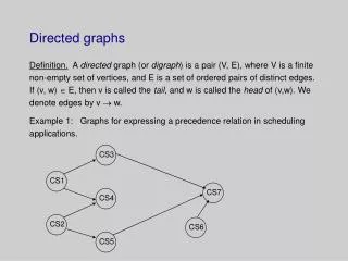
CS1 CS2 CS4 CS3 CS7 CS6 CS5 Directed graphs Definition. A directed graph (or digraph) is a pair (V, E), where V is a finite non-empty set of vertices, and E is a set of ordered pairs of distinct edges. If (v, w) E, then v is called the tail, and w is called the head of (v,w). We denote edges by v w. Example 1: Graphs for expressing a precedence relation in scheduling applications.
In Example 1, the precedence relation must satisfy the following conditions: • Irreflexivity, i.e. for all s S, s -/-> s. • Asymmetry, i.e. for all s, t S, if s t, then t -/-> s. • Transitivity, i.e. for all s, r, t S, if r s and s t, then r t. where S is a set of vertices. Property: In a directed acyclic graph, for all s, t S, s t iff there is a path from s to t.
10 2 4 3 7 5 6 1 8 9 Example 2. Graph for expressing a binary relation. Let S = {1, 2, 3, 4, 5, 6, 7, 8, 9, 10}, and R: y x iff x y and x divides y.
Depth-first search in directed graphs Same as in undirected graphs, but the result is a depth-first search forest, rather than a tree. Example to be distributed in class.
Transitive closure of a graph The problem: Given a directed graph, G = (V, E), find all of the vertices reachable from a given starting vertex v V. Transitive closure (definition): Let G = (V, E) be a graph, where x y, y z (x, y, z V). Then we can add a new edge x z. A graph containing all of the edges of this nature is called the transitive closure of the original graph. The best way to represent the transitive closure graph (TCG) is by means of an adjacency matrix. To generate the TCG, we can use the Warshall's algorithm: for y := 1 to NumberOfNodes { for x := 1 to NumberOfNodes { if A[x,y] then { for z := 1 to NumberOfNodes if A[y,z] then A[x,z] := True } } } Efficiency result: Warshall's algorithm solves the transitive closure problem in O(NumberOfNodes^3) time. Example to be distributed in class.
1 2 3 The all shortest path problem The problem: Given a weighted directed graph, G = (V, E, W), find the shortest path between all pairs of vertices from V. Solution 1: Run Dijkstra's shortest path algorithm V^2 times, each time with a new starting and destination vertex. The overall efficiency of this solution will be O(NumberOfNodes^4). Solution 2: Floyd's all-pairs shortest path algorithm. Example. Distance matrix: 1 2 3 1 0 8 5 2 3 0 3 2 0 5 8 2 3
Example (contd.) The distance matrix is computed as follows: 0, if i = j. Distance[i, j] = EdgeWeight(i, j). , otherwise. Floyd's algorithm computes a sequence of distance matrices, such that at each step k of the computation process (1 k NumberOfNodes), Distance[i,j] satisfies the following two criteria: • The path starts at vertex i, and ends at vertex j. • Internal vertices on the path come from the set of vertices having index values between 1 and k inclusive. In our example, the computation process is carried out as follows: Step 1: Consider all paths, which contain node 1 as an internal node, i.e. 2 --> 1 --> 3 1 2 3 W(2,1) = 3 1 0 8 5 W(1,3) =5 2 3 0 8 d(2,3) = 8 < 3 2 0
Example (contd.) Step 2: Consider all paths, which contain node 2 as an internal node, i.e. 3 --> 2 --> 1 1 2 3 W(3,2) = 2 1 0 8 5 W(2,1) = 3 2 3 0 8 3 5 2 0 d(3,1) = 5 < Step 3: Consider all path, which contain node 3 as an internal node, i.e. 1 --> 3 --> 2 1 2 3 W(1,3) = 5 1 0 7 5 W(3,2) = 2 2 3 0 8 3 5 2 0 d(1,2) = 7 < 8
Floyd's algorithm (contd.) for k := 1 to NumberOfNodes { for i := 1 to NumberOfNodes { for j := 1 to NumberOfNodes { Distance[i,j] := min (Distance[i,j], Distance[i,k] + Distance[k,j]) } } } Efficiency result: Floyd's algorithm solves the all shortest paths problem in O(NumberOfNodes^3) time.
CS3 CS1 CS2 CS4 CS7 CS6 CS5 Topological ordering on directed acyclic graphs The problem: Given a directed acyclic graph (DAG), G = (V, E), define a linear sequence in which graph nodes can be visited. Example. Here such sequences are: • CS1 CS2 CS3 CS4 CS5 CS6 CS7 These are called “topological • CS2 CS1 CS5 CS4 CS3 CS6 CS7 orderings” of the graph’s nodes. • CS6 CS2 CS5 CS1 CS1 CS3 CS7 • and so on…
Definition. The indegree of a graph node is the number of edges entering the node, and the outdegree of a graph node is the number of edges exiting from the node. Topological ordering algorithm: ComputeInitialIndegree (G, Indegree) for n := 1 to NumberOfNodes if Indegree[n] = 0 then enqueue (ZeroQ, n) orderCount := 0 while (! Empty (ZeroQ)) { v := dequeue(ZeroQ) orderCount := orderCount + 1; T[orderCount] := v for n := 1 to NumberOfNodes if (edge (v, n)) then Indegree[n] := Indegree[n] – 1 if (Indegree[n] = 0) then enqueue(ZeroQ) Efficiency result: ComputeInitialIndegree is O(NumberOfNodes^2) operation, therefore total efficiency of topological ordering is O(NumberOfNodes^2).