Download

1 / 50
510 likes | 550 Views
Exploring the properties of Directed Acyclic Graphs (DAGs) including Bayesian Networks, Conditional Independence, Markov Equivalence, and Faithfulness. Understand the implications of Greedy Equivalence Search, I-Map, and Factorization within this framework.

E N D
Markov Properties of Directed Acyclic Graphs Peter Spirtes
Outline • Bayesian Networks • Simplicity and Bayesian Networks • Causal Interpretation of Bayesian Networks • Greedy Equivalence Search
Outline • Bayesian Networks • Simplicity and Bayesian Networks • Causal Interpretation of Bayesian Networks • Greedy Equivalence Search
Directed Acyclic Graph (DAG) ng bl ng – no gas bl – battery light on bd bd – battery dead ns – no start ns • The vertices are random variables. • All edges are directed. • There are no directed cycles.
Definition of Conditional Independence • Let P(X,Y,Z) be a joint distribution over X, Y, Z. • X is independent of Y conditional on Z in P, written as IP(X,Y|Z), if and only if P(X|Y,Z) = P(X|Z) whenever P(y,z) > 0.
Probabilistic Interpretation - Local Markov Condition • Distribution P satisfies the Local Markov Condition for DAG G iff each vertex is independent in P of all vertices that are neither parents nor descendants, conditional on its parents. ng bl bd ns IP(ng,{bd,bl}|∅) IP(bl,{ng,ns}|bd) IP(bd,ng|∅) IP(ns,bl|{bd,ng}
Probabilistic Interpretation: I-Map • If distribution P satisfies the Local Markov Condition for G, G is an I-map (Independence-map) of P. ng bl bd ns
Graphical Entailment • If G being an I-map of P entails a conditional independence relation I holds in P, G entails I. • Examples: In every distribution P that G is an I-map of • IP(bd,ng|∅) • IP(bl,ng|{bd,ns}) ng bl bd ns
If I is Not Entailed by G • If conditional independence relation I is not entailed by G, then I may hold in some (but not every) distribution P that G is an I-map of. • Example: G is an I-map of some P such that ~IP(ns,bl|∅) and some P’ such that IP’(ns,bl|∅) ng bl bd ns
Factorization ng bl bd ns • If G is an I-map of P, then P(ng,bd,bl,ns) = P(ng)P(bd)P(bl|bd)P(ns|bd,ng)
Example of Parametric Family ng bl bd ns • P(ng = 0) • P(bd = 0) • P(bl = 0|bd = 0) • P(bl = 0|bd = 1) • P(ns = 0|ng = 0, bd = 0) • P(ns = 0|ng = 0, bd = 1) • P(ns = 0|ng = 1, bd = 0) • P(ns = 0|ng = 1, bd = 1) • For binary variables, the dimension of the set of distributions that G is an I-map of, is 8.
Outline • Bayesian Networks • Simplicity and Bayesian Networks • Causal Interpretation of Bayesian Networks • Greedy Equivalence Search
Markov Equivalence • Two DAGs G1 and G2 are Markov equivalent when they contain the same variables, and for all disjoint X, Y, Z, X is entailed to be independent from Y conditional on Z in G1 if and only if X is entailed to be independent from Y conditional on Z in G2
Markov Equivalence • Two DAGS over the same set of variables are Markov equivalent iff they have: • the same adjacencies • the same unshielded colliders (X → Y ← Z, and no X → Z or Z→ X edge)
Markov Equivalence ng bl bd ns ng bl bd ns DAG G’ DAG G
Patterns • A pattern represents a Markov equivalence class of DAGs. ng bl bd ns ng bl bd ns ng bl bd ns Pattern(G) DAG G’ DAG G
Patterns • The adjacencies in a pattern are the same as the adjacencies in each DAG in the d-separation equivalence class. • An edge is oriented as A → B in the pattern if it is oriented as A → B in every DAG in the equivalence class. • An edge is oriented as A – B in the pattern if the edge is oriented as A → B in some DAGs in the equivalence class, and as A ← B in other DAGs in the equivalence class.
Patterns • All of the conditional independence relations entailed by a DAG G represented by a pattern G’ can be read off of G’. • So we can speak of a pattern being an I-map of P by extension.
Faithfulness • P is faithful to G if • Every conditional independence entailed by G, is true in P (Markov) • Every conditional independence true in P is entailed by G • For every P, there is at most one, but possibly no pattern that P is faithful to.
Unfaithfulness X Y Z G • + IP(X,Z|∅) • IP(X,Z|∅) • Both G and G’ are patterns that are I-maps of a P in which the only independence is I(X,Z|∅), but P is faithful only to G’, not G. X Y Z G’
Unfaithfulness • IP(X,Z|Y) + IP(X,Z|∅) • IP(X,Z|Y) + IP(X,Z|∅) • If both IP(X,Z|Y) + IP(X,Z|∅) then P is not faithful to any DAG. X Y Z X Y Z
Violations of Faithfulness • If conditional independence can be expressed as rational function of the parameters (e.g. any exponential family including Gaussian and multinomial) then violations of faithfulness are Lebesgue measure 0.
Minimality • G is Markov and Minimal for P if and only if • Every conditional independence entailed by G is true in P (Markov) • No graph that entails a subset of the conditional independencies entailed by G is Markov to P (minimality). • For every P, there is at least one, and possibly more than one pattern, Markov and minimal for P.
Two Markov Minimal Graphs for P • IP(X,Z|Y) + IP(X,Z|∅) • IP(X,Z|Y) + IP(X,Z|∅) X Y Z X Y Z
Faithfulness and Minimality • If P is faithful to G, then G is a unique Markov Minimal pattern for P.
Lattice of I-maps Dimensionality → Entailment Inclusion → X Y Z X Y Z X Y Z X Y Z X Y Z X Y Z X Y Z X Y Z X Y Z X Y Z X Y Z
Outline • Bayesian Networks • Simplicity and Bayesian Networks • Causal Interpretation of Bayesian Networks • Greedy Equivalence Causal Search
Causal Interpretation of DAG • There is an edge X → Y in G if and only if there is some pair of experimental manipulations of all of the variables in G other than Y, that • differ only in what manipulation is performed on X; and • make the probability of Y different.
Causal Sufficiency • A set S of variables is causally sufficient if there are no variables not in S that are direct causes of more than one variable in S.
Causal Sufficiency ng bl bd ns • S = {ng, ns} is causally sufficient. • S = {ng, ns, bl} is not causally sufficient.
Causal Markov Assumption • In a population Pop with causally sufficient graph G and distribution P, each variable is independent of its non-descendants (non-effects) conditional on its parents (immediate causes) in P. • Equivalently: G is an I-map of P.
Causal Faithfulness Assumption • In a population Pop with causally sufficient graph G and distribution P, I(X,Y|Z) in P only if X is entailed to be independent of Y conditional on Z by G.
Causal Faithfulness Assumption • As currently used, it is a substantive simplicity assumption, not a methodological simplicity assumption. It says to prefer the simplest explanation: if a more complicated explanation is true, it leads astray.
Causal Faithfulness Assumption • It serves two roles in practice: • Aiding model choice (in which case weaker versions of the assumption will do) • Simplifying search
Causal Minimality Assumption • In a population Pop with causally sufficient graph G and distribution P, G is a minimal I-map of P.
Causal Minimality Assumption • This is a strictly weaker simplicity assumption than Causal Faithfulness. • Given the manipulation interpretation of the causal graph, and an everywhere positive distribution, the Causal Minimality Assumption is entailed by the Causal Markov Assumption.
Outline • Bayesian Networks • Simplicity and Bayesian Networks • Causal Interpretation of Bayesian Networks • Greedy Equivalence Search
Greedy Equivalence Search • Inputs: Sample from a probability distribution over a causally sufficient set of variables from a population with causal graph G. • Output: A pattern that represents G.
Assumptions • Causally sufficient set of varaibles • No feedback • The true causal structure can be represented by a DAG. • Causal Markov Assumption • Causal Faithfulness Assumption
Consistent scores • If model M1 contains the true distribution, while model M2 doesn’t, then in the large sample limit M1gets the higher score. • If both M1 and M2contain the true distribution, and M1 has fewer parameters than M2 does, then in the large sample limit M1gets the higher score.
Consistent scores • So, assuming the Causal Markov and Faithfulness conditions, a consistent score assigns the true model (and its Markov equivalent models) the highest score in the limit. • Examples: Bayesian Information Criterion, posterior of Bde or Bge prior
Score Equivalence • Under BIC, Bde, and Bge, Markov equivalent DAGs are also score equivalent, i.e., always receive the same score. (Could also use posterior probabilities under a wide variety of priors). • This allows GES to search over the space of patterns, instead of the space of DAGs.
Two Phases of GES • Forward Greedy Search (FGS): Starting with any pattern Q, evaluate all patterns that are I-maps of Q with one more edge, and move to the one with the best increase of score. Iterate until local maximum. • Backward Greedy Search (BGS): Starting with a pattern Q that contains the true distribution, evaluate all patterns with one fewer edge of which Q is an I-map, and move to the one with the best increase of score. Iterate until local maximum.
Asymptotic Optimality • In the large sample limit, GES always returns a pattern that is minimal and Markov to P. • Proof. Because the score is consistent, the forward phase continues until it reaches a pattern G such that P is Markov to G. The backward phase preserves Markov, and continues until there is no pattern that is both Markov to P and entails more independencies.
Asymptotic Optimality • If P is faithful to the causal pattern G, then BGS returns G. • Proof Sketch: G is the unique pattern that is minimal and Markov to P. By the previous theorem, GES returns G.
When GES Fails to Find the Right Causal Pattern • In the large sample limit, GES always finds a Markov Minimal pattern • Some Markov Minimal pattern may not be the true causal pattern if • Causal Minimality Assumption is violated; or • There are multiple Markov Minimal patterns, and GES outputs the wrong one
One Markov Minimal Pattern for P, but Not the Causal Pattern X Y Z • + I(X,Z|∅) • I(X,Z|∅) X Y Z
Two Markov Minimal Graphs for P • I(X,Z|Y) + I(X,Z|∅) • I(X,Z|Y) + I(X,Z|∅) X Y Z G X Y Z G’ • For some parametric families G and G’ have the same score and the same dimension. • For other parametric families, G’ has lower dimension and higher score than G.
Multiple Minimal I-maps? • Lower Standard of Success • Output all Markov Minimal • Output any Markov Minimal • More Data • Experiments • More Background Knowledge • Time order, etc.
References • Chickering, M. (2002) Optimal Structure Identification With Greedy Search, Journal of Machine Learning Research3, pp. 507-554. • Spirtes, P., Glymour, C., and Scheines, R., (2000) Causation, Prediction, and Search, 2nd edition. MIT Press, Cambridge, MA.