Hopfield NNets
830 likes | 1.05k Views
Hopfield NNets. N. Laskaris. Professor John Hopfield The Howard A. Prior Professor of Molecular Biology Dept. of Molecular Biology Computational Neurobiology; Biophysics Princeton University.

Hopfield NNets
E N D
Presentation Transcript
Hopfield NNets N. Laskaris
Professor John Hopfield The Howard A. Prior Professor of Molecular Biology Dept. of Molecular Biology Computational Neurobiology; Biophysics Princeton University
The physicist Hopfield showed that models of physical systems could be used to solve computational problems Such systems could be implemented in hardware by combining standard components such as capacitors and resistors.
The importance of the Hopfield nets in practical application is limited due to theoretical limitations of the structure, but, in some cases, they may form interesting models.
Usually employed in binary-logic tasks : e.g. pattern completion and association
In the beginning of 80s Hopfield published two scientific papers, which attracted much interest. (1982):‘’Neural networks and physical systems with emergent collective computational abilities’’.Proceedings of the National Academy of Sciences, pp. 2554-2558. (1984):‘’Neurons with graded response have collective computational properties like those of two-state neurons’’.Proceedings of the National Academy of Sciences, pp. 81:3088-3092 This was the starting point of the new era of neural networks, which continues today
‘‘The dynamics of brain computation” The core question : How is one to understand the incredible effectiveness of a brain in tasks such as recognizing a particular face in a complex scene?
Like all computers, a brain is a dynamical system that carries out its computations by the change of its 'state' with time. Simple models of the dynamics of neural circuits are described that have collective dynamical properties. These can be exploited in recognizing sensory patterns. Using these collective properties in processing information is effective in that it exploits thespontaneousproperties of nerve cells and circuits to produce robust computation.
J. Hopfield’s quest While the brain is totally unlike modern computers, much of what it does can be described as computation. Associative memory, logic and inference, recognizing an odor or a chess position, parsing the world into objects, and generating appropriate sequences of locomotor muscle commands are all describable as computation. His research focuses on understanding how the neural circuits of the brain produce such powerful and complex computations.
The simplest problem in olfaction is simply identifying a known odor. Olfaction However, olfaction allows remote sensing, and much more complex computations involving wind direction and fluctuating mixtures of odors must be described to account for the ability of homing pigeons or slugs to navigate through the use of odors. Hopfield has been studying how such computations might be performed by the known neural circuitry of the olfactory bulb and prepiriform cortex of mammals or the analogous circuits of simpler animals.
Dynamical systems Any computer does its computation by its changes in internal state. In neurobiology, the change of potentials of neurons (and changes in the strengths of the synapses) with time is what performs the computations. Systems of differential equations can represent these aspects of neurobiology. He seeks to understand some aspects of neurobiological computation through studying the behavior of equations modeling the time-evolution of neural activity.
Action potential computation For much of neurobiology, information is represented by the paradigm of ‘‘firing rates’’, i.e. information is represented by the rate of generation of action potential spikes, and the exact timing of these spikes is unimportant.
Action potential computation Since action potentials last only about a millisecond, the use of action potential timing seems a powerful potential means of neural computation.
Action potential computation There are cases, for examplethe binaural auditory determination of the location of a sound source, where information is encoded in the timing of action potentials.
Speech Identifying words in natural speech is a difficult computational task which brains can easily do. They use this task as a test-bed for thinking about the computational abilities of neural networks and neuromorphic ideas
Simple (e.g. binary-logic ) neurons are coupled in a system with recurrent signal flow
A 2-neurons Hopfield network of continuous states characterized by 2 stable states 1st Example Contour-plot
2nd Example A 3-neurons Hopfield network of 23=8 states characterized by 2 stable states
3rd Example Wij = Wji The behavior of such a dynamical system is fully determined by the synaptic weights And can be thought of as an Energy minimization process
Hopfield Nets are fully connected, symmetrically-weighted networks that extended the ideas of linear associative memories by adding cyclic connections . Note: no self-feedback !
Operation of the network After the ‘teaching-stage’, in which the weights are defined, the initial state of the network is set (input pattern) and a simple recurrent rule is iterated till convergence to a stable state (output pattern) Regarding training a Hopfield net as a content-addressable memory the outer-product rule for storing patterns is used There are two main modes of operation: Synchronous vs.Asynchronousupdating
Hebbian Learning Probe pattern Dynamical evolution
A Simple Example Step_1.Design a network with memorized patterns (vectors)[ 1, -1, 1 ] & [ -1, 1, -1 ]
#1: y1 #2: y2 #3: y3 Step_2. Initialization There are 8 different states that can be reached by the net and therefore can be used as its initial state
Step_3. Iterate till convergence 3 different examples of the net’s flow - Synchronous Updating - It converges immediately
Step_3. Iterate till convergence Stored pattern - Synchronous Updating - Schematic diagram of all the dynamical trajectories that correspond to the designed net.
Or Step_3. Iterate till convergence - Asynchronous Updating - Each time, select one neuron at random and update its state with the previous rule and the –usual- convention that if the total input to that neuron is 0 its state remains unchanged
Explanation of the convergence There is an energy function related with each state of the Hopfield network E( [y1, y2, …, yn]T ) = -Σ Σ wij yiyj where [y1, y2, …, yn]T is the vector of neurons’ output, wijis the weight from neuron j toneuron i, and the double sum is over i and j.
The corresponding dynamical system evolves toward states of lower Energy
States of lowest energy correspond to attractors of Hopfield-net dynamics Attractor-state E( [y1, y2, …, yn]T)= = -Σ Σ wij yiyj
Capacity of the Hopfield memory In short, while training the net (via the outer-product rule) we’re storing patterns by posing different attractors in the state-space of the system. While operating, the net searches the closest attractor. When this is found, the corresponding pattern of activation is outputted
How many patterns we can store in a Hopfield-net ? 0.15 N,N: # neurons
Computer Experimentation Class-project A simple Pattern Recognition Example
Perfect Recall- Image Restoration Erroneous Recall
Irrelevant results Note: explain the ‘negatives’ ….
The continuous Hopfield-Net as optimization machinery
[ Tank and Hopfield ; IEEE Trans. Circuits Syst. 1986; 33: 533-541.]: ‘Simple "Neural" Optimization Networks: An A/D Converter, Signal Decision Circuit, and a Linear Programming Circuit’
Hopfield modified his network so as to work with continuous activation and -by adopting a dynamical-systems approach- showed that the resulting system is characterizedby a Lyaponov-function who termed it ‘Computational-Energy’& which can be used to tailor the net for specific optimizations
The system of coupled differential equation describing the operation of continuous Hopfield net Neuronal outputs: Yi≡ Vi Biases: Ii Weights: Wij ≡ Tij Tij=Tji και Tij=0 The Computational Energy
When Hopfield nets are used for functionoptimization, the objective function Fto be minimized is written as energy functionin the form of computational energy E . The comparison betweenE and Fleadsto the design, i.e. definition of links and biases, of the networkthat can solve the problem.
The actual advantage of doing this is that the Hopfield-net has a direct hardware implementation that enables even a VLSI-integration of the algorithm performing the optimization task
An example: ‘Dominant-Mode Clustering’ Given a set of N vectors {Xi} define the k among them that form the most compact cluster {Zi} The objective function F can be written easily in the form of computational energy E
There’s an additional Constraint so as kneurons are ‘on’ With each pattern Xi we associate a neuron in the Hopfield network ( i.e. #neurons = N ). The synaptic weights are the pairwise-distances (*2) If its activation is ‘1’ when the net will converge the corresponding pattern will be included in the cluster.
A classical example: ‘The Travelling Salesman Problem’