Distribution Planning for Efficient Supply Chain Management

1. MGTSC 352 QUIZ 3 NOTES

2. Distribution Planning • What should overall distribution system be? • Where should inventories of products or raw materials be stored? • How much inventory of each product and raw material should be stored at each location • How should the flow of products and raw materials through the distribution be coordinated • What models of transportation should be used?

3. Distribution Planning • All distribution problems are really special case of minimum cost problem, even the shortest distance problem, which replaces distances with cost • Remember to freeze cells when using the sumif function • Hit ctrl + ~ to get into formula mode, will make it much easier to debug

4. Distribution Planning

5. Distribution Planning • Shortest path problem • If we are required to go to a certain path, best way is to solve it in two parts • 1st part is when we go from supply city to intermediate path • 2nd part is when we go from intermediate city to final demand path • Set demand = 1 at destination city and set supply = 1 at city of origin • Make sure that supply + flowin = demand + flow out • This will allow us to make a path with no jumps

6. Distribution Planning • Shortest Path problem cont. • If we have to traverse a specific arc, but not to a specific city to within that arc, before going to a specific city, make sure you allow for two-way travel • In three cells, have: • city 1 -> city 2 • City 2 -> city 1 • sum • Each path will reference truckload along that path • Sum is the sum of the two arcs • Constrain solver so that the sum>=1, that way it must traverse the path but also allows for back travel

7. Distribution Planning • New locations • If wondering whether or not to open a new facility, use a binary variable • To ensure that we don’t produce if we don’t open: • Set an upper bound = max prod * binary • Constrain solver so that production can not be greater than the upper bound • Must constrain solver so that supply + flow in + production >= demand + flow out

8. Inventory Management • Goods that have not yet been sold • Keep inventory when • Demand unpredictable • Delivery takes time • Fixed cost for delivery • Relevant question • When to order (ROP = Reorder point) • How much to order (Q = reorder quantity) • MAKE SURE TIME UNITS ARE CONSISTENT, DON’T MIX YEARS WITH MONTHS

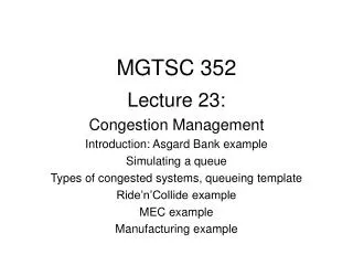
9. Acquisition cost ($/unit purchased) Ordering costs($/order) clerical expenses delivery, inspection setup (prod.) Carrying costs = Holding costs($/unit/time unit) cost of capital insurance shrinkage, spoilage, obsolescence material handling (fork lifts, space) Shortage costs($/unit short) lost goodwill, discounts, penalties lost sales shut down of assembly line (prod.) Relevant Costs

10. Maximum inventory Avg. inventory ROP Q Leadtime Minimum inventory Inventory LTD = Demand during leadtime Time

11. Histogram Need 3 columns • # sold, bins, and frequency as headers • # sold will be a range (0-2, 3-4, etc..) • Bins refers to values at or below that value • 2 means 0-2, 4 means 3-4, etc.. • Frequency means how often value corresponding to a bin shows up in the dataset

12. Histogram • Highlight the empty frequency cells • Type in frequency (data, bins) • While they are all highlighted, hit ctrl + shift + enter, this will cause the frequency to appear in the cells

13. Histogram • in the graph template, hit column graph • Highlight # sales and frequency to be graphed • Once graph is made, double click the graph and under options you can change the distance between the columns to be 0 • Histogram complete

14. Simulation • Orders take time to come into your place of business, this time will affect how your business is run because it will effect your reorder points and order quantities • Beginning inventory is equal to ending inventory of the previous day + the order that came in that day

15. Simulation • Inventory position is beginning inventory plus inventory that is in transit. If we ordered two day ago, and we know we will get the inventory in 5 days, then we wouldn’t order more stock because we know that we have an order on the way • If a new order just arrives and it is too short, then we would put a new order through

16. Simulation • Order if demand is greater than the inventory position • We can use if statements to ensure this • If(demand>=inventory position, order amount Q, else don’t place order) • Sales will be the minimum of demand or beginning inventory, not inventory position because that inventory is not in the store • Min(demand, beginning inventory)

17. Simulation • Shortage is demand less sales • Ending inventory is beginning inventory less sales. If your order will come in at the end of the business day, then ending inventory will include this as well • Holding cost is the average of beginning and ending inventory, multiplied by the holding cost per unit

18. Simulation • Fill rate is the amount of demand that is satisfied by the inventory • =total sales/total demand

19. Tables in Excel • Say we want to see how net profit varies with differing ROP and Q • Put values for ROP and Q along row and column, except leave the top left corner of the table blank • In the top left corner, reference net profit • Highlight entire area, then go data->table • For row, reference original value for row, and for column, reference original value for column • Can use conditional formatting to highlight the max amount or to highlight minimum amounts, if you require that we must reach a certain profit, or fill rate or whatever

20. EOQ = Economic Order Quantity • Assumptions • Demand is constant • Inventory drops to zero just before an order arrives • Variables: • S = order cost ( per order) • H = carrying cost (per item per order) • D = annual demand • Order cost = (D/Q)/S; Carrying Cost = (Q/2)*H Q* = sqrt(2DS/H) • Q* = quantity to order that will minimize cost under the EOQ model

21. EOQ = Economic Order Quantity • Simulation modeling is a flexible modeling approach that is capable of replicating the real world intricacies of an inventory system but it is also generally an expensive (time and money) approach. In the previous worksheet we used a historical simulation to find a good policy (values for Q and ROP). We found the policy by trial and error, facilitated by a two-way data table. • We will use a simpler approximate two-step analytical method to first find Q and then find ROP. We use the well-known EOQ model (which trades off ordering costs with holding costs) to find Q. Then we use this Q and an estimate of the probability distribution of demand during the lead time to determine ROP, either by meeting a pre-specified level of service or fill rate or by minimizing the costs of incurring a shortage plus the cost of carrying extra safety stock). This two-step method involves many approximations, but in practice it usually gives a near-optimal policy • Find Q*, then use LTD (lead time demand model) to find ROP using Q from previous step.

22. pg. 151 Simulation versus EOQ

23. LTD – Lead time demand • Lead time = how long we wait while receiving an order • Lead time demand = how much demand would occur while we are waiting for our order to arrive • Goal is to reduce the probability of shortages

24. LTD – Lead time demand • Set the lead time • LTD will be the sum of the demand for the lead time • Shortage will occur if LTD>=ROP • If(LTD>=ROP,LTD-ROP,0) • For shortage per cycle • cycle= demand/Q • Shortage = cycle*average shortages/year • Fill rate • = sales/demand • = (demand-shortages)/demand