Download
1 / 24
250 likes | 412 Views
MGTSC 352. Lecture 23: Congestion Management Introduction: Asgard Bank example Simulating a queue Types of congested systems, queueing template Ride’n’Collide example MEC example Manufacturing example. Analyzing a Congested System (pg. 174). Inputs. System Description.

E N D
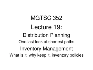
MGTSC 352 Lecture 23: Congestion Management Introduction: Asgard Bank example Simulating a queue Types of congested systems, queueing template Ride’n’Collide example MEC example Manufacturing example
Analyzing a Congested System (pg. 174) Inputs System Description Model of the System Measures of Quality of Service Outputs Measures important to Servers
pg. 168 Asgard Bank: Times Between Arrivals(pg. 173)
Including Randomness: Simulation • Service times: Normal distribution, mean = 57/3600 hrs, stdev = 10/3600 hrs. MAX(NORMINV(RAND(),57/3600,10/3600),0) • Inter-arrival times: Exponential distribution, mean = 1/ 60 hrs. – (1/60)*LN(RAND()) To Excel …
71 arrivals Simulated Lunch Hour 1:
50 arrivals Simulated Lunch Hour 2:
Unused capacity Simulated Lunch Hour 3:
Causes of Congestion • Higher than average number of arrivals • Lower than average service capacity • Lost capacity due to timing Lesson: For a service where customers arrive randomly, it is not a good idea to operate the system close to its average capacity
Template.xls • Does calculations for • M/M/s • M/M/s/s+C • M/M/s//M • M/G/1 • Want to know more? Go to http://www.bus.ualberta.ca/aingolfsson/qtp/ • Asgard Bank Data • Model: M/G/1 • Arrival rate: 1 per minute • Average service time: 57/60 min. • St. dev of service time: 10/60 min.
Asgard Conclusions • The ATM is busy 95% of the time. • Average queue length = 9.3 people • Average no. in the system = 10.25(waiting, or using the ATM) • Average wait = 9.3 minutes • What if the service rate changes to … • 1.05 / min.? • 1.06 / min.?
Ride’n’Collide (pg. 178) • Repair personnel cost: $10 per hour • Average repair duration: 30 minutes • Lost income: $50 per hour per car • Number of cars: 20 cars • A car will function for 10 hours on average from the time it has been fixed until the next time it needs to be repaired. • How many repair-people should be hired?
Ride’n’Collide • Customers = • Servers = • Average number in system = • Lost revenue per hour = • Arrival rate = • Service rate = • Model to use:
Waiting Line Analysis Template:Which Model to Use? • Who are the customers? • Who are the servers? • Where is the queue? … not always obvious
waiting room = queue parallel servers potential customers • If you are told how many customers there are … then you should consider using the “finite population” template Number is small enough to worry about
waiting room = queue parallel servers potential customers • If you are told the maximum number of customers that can wait (the size of the waiting room) … then you should consider using the “finite Q” template Capacity is small enough to worry about
If you are told the standard deviation of the service times, and there is 1 server … then you should consider using the “MG1” template waiting room = queue one server, non-exponential service time distribution potential customers
If you are told nothing about the size of the pool of potential customers, or the maximum number that will wait, or the standard deviation of the service times, … then you should probably use the “MMs” template
MEC (p. 181) • One operator, two lines to take orders • Average call duration: 4 minutes exp • Average call rate: 10 calls per hour exp • Average profit from call: $24.76 • Third call gets busy signal • How many lines/agents? • Line cost: $4.00/ hr • Agent cost: $12.00/hr • Avg. time on hold < 1 min.
Modeling Approaches • Simulation • Waiting line analysis template • We’ll use both for this example To Excel …
Manufacturing Example (p. 184) Machine (1.2 or 1.8/minute) 1/minute Poisson arrivals Exponential service times
Manufacturing Example • Arrival rate for jobs: 1 per minute • Machine 1: • Processing rate: 1.20/minute • Cost: $1.20/minute • Machine 2: • Processing rate: 1.80/minute • Cost: $2.00/minute • Cost of idle jobs: $2.50/minute • Which machine should be chosen? To Excel …
Manufacturing Example • Cost of machine 1 = $1.20 / min. + ($2.50 / min. / job) (5.00 jobs) = $13.70 / min. • Cost of machine 2 =$2.00 / min. + ($2.50 / min. / job) (1.25 jobs) = $5.13 / min. Switching to machine 2 saves money – reduction in lost revenue outweighs higher operating cost.
Cost of waiting (Mach. 1) • Method 1: • Unit cost × L = ($2.50 / min. job) (5.00 jobs) = $13.70 / min • Method 2: • Unit cost ×× W = = ($2.50 / min. job) (5.00 min) (1 job/min) = $13.70 / min • Little’s LawL = × W