Importance sampling for MC simulation (“Importance-weighted random walk”)

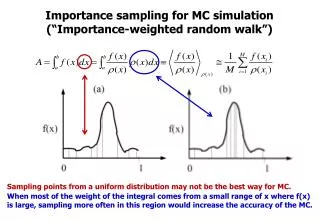
1. Importance sampling for MC simulation (“Importance-weighted random walk”) Sampling points from a uniform distribution may not be the best way for MC. When most of the weight of the integral comes from a small range of x where f(x) is large, sampling more often in this region would increase the accuracy of the MC.

2. Example: Importance of small region: Measuring the depth of the Nile Systematic quadrature or uniform sampling Importance sampling (importance weighted random walk) Frenkel and Smit, Understanding Molecular Simulations

3. Example: Importance of small region: Energy funnel in protein folding • Cyrus Levinthal formulated the “Levinthal paradox” (late 1960’s): • Consider a protein molecule composed of (only) 100 residues, • each of which can assume (only) 3 different conformations. • The number of possible structures of this protein yields 3100 = 5×1047. • Assume that it takes (only) 100 fs to convert from one structure to another. • It would require 5×1034 s = 1.6×1027 years to ”systematically” explore all possibilities. • This long time disagrees with the actual folding time (μs~ms).  Levinthal’s paradox

4. To decrease the error of MC simulation ~ cost  (f) = standard deviation in the observable O, i.e., y = f(x), itself fmeasures how much f(x) deviates from its average over the integration region. ~ independent of the number of trials M (or N) ~ estimated from one simulation fluctuating, varying function sharp (probability) distribution O=f(x) O O=f(x) O broad distribution flat function f f <f> <f> A A vs. x2 xi x1 xM x a b p(O) x p(O) 0 1 a b 0 1 (f = 0) (f > 0) non-ideal, real case the ideal case Importance sampling

5. Importance sampling for MC simulation: Example From N-step uniform sampling 3 in accuracy From normalized importance sampling weighted by w(x)

6. Lab 3: Importance sampling for MC simulation

7. What’s new in Lab 3: Importance sampling * Include “cpu.h”, compile “cpu.c”, and call “cpu()” to measure the cpu time of the run. tstart = cpu(); ~ tend = cpu(); printf("CPU time: %5.5f s, CPU time/measure: %g s", tend - tstart, (tend - tstart) / M); * Calculate the normalization constant N for each probability distribution function (x). * Include “ran3.h” & “fran3.h”; compile fran3.c; call “fexp” or “flin” defined in fran3. r = ran3(&seed); f_x = exp(-x*x); r = ran3(&seed); rho = fexp(r, &x); f_x = exp(-x*x) / rho; r = ran3(&seed); rho = flin(r, &x); f_x = exp(-x*x) / rho; * Display histograms for the distribution of x values generated by fran3 (for the step 4 only). r = ran3(&seed); f_x = exp(-x*x); i_hist = (int) (x * inv_dx); if (i_hist < n_hist) hist[i_hist] += 1.0; r = ran3(&seed); rho = fexp(r, &x); f_x = exp(-x*x) / rho; i_hist = (int) (x * inv_dx); if (i_hist < n_hist) hist[i_hist] += 1.0; r = ran3(&seed); rho = flin(r, &x); f_x = exp(-x*x) / rho; i_hist = (int) (x * inv_dx); if (i_hist < n_hist) hist[i_hist] += 1.0;

8. * Display histograms for the distribution of x values generated by fran3. (full version) /* number of bins in histogram*/ n_hist = 50; /* Allocate memory for histogram */ hist = (double *) allocate_1d_array(n_hist, sizeof(double)); /* Initializae histogram */ for (i_hist = 0; i_hist < n_hist; ++i_hist) hist[i_hist] = 0.0; /* Size of the ihistogram bins */ dx = 1.0 / n_hist; /* 1.0 is the size of the interval */ inv_dx = 1.0 / dx; /* histogram accumulated */ i_hist = (int) (x * inv_dx); if (i_hist < n_hist) hist[i_hist] += 1.0; /* Write histogram. */ fp = fopen("hist_2.dat", "w"); for (i_hist = 0; i_hist < n_hist; ++i_hist) { x = (i_hist + 0.5) * dx; fprintf(fp, "%g %g", x, hist[i_hist] / M); } fclose(fp); Plot with gnuplot, excel, origin, … Fit to a function. What is the resulted function?

9. Furtherreading: Sampling a non-uniform & discrete probability distribution {pi} (towersampling) (Ref) Gould, Toboshnik, Christian, Ch. 11.5

10. Furtherreading: Sampling a non-uniform & continuous probability distribution (x)

11. Example

15. Lab 3: Importance sampling for MC simulation bad distribution function w(x) (x) p(x) Normalized! constant distribution function (uniform) Normalized! good distribution function Normalized! Integrand f(x)

16. Results: Importance sampling for MC simulation One experimentwith M measures n = 100 experiments, eachwith M measures

17. Results: Importance sampling for MC simulation One experimentwith M measures n = 100 experiments, eachwith M measures

18. Importance sampling = Importance-weighted average Analogy: Throw a dice with the results of {1, 2, 2, 2, 2, 4, 5, 6}. (Discrete) probability distribution {pi, i=1-6} = {1, 4, 0, 1, 1, 1} / 8 where 8 = 1+4+0+1+1+1 = {1/8, 1/2, 0, 1/8, 1/8, 1/8} Mean value <A> = 3 = 24/8 = (1+2+2+2+2+4+5+6) / 8 = (1 + 2x4 + 4 + 5 + 6) / 8 = 1x1/8 + 2x4/8 + 3x0/8 + 4x1/8 + 5x1/8 + 6x1/8

19. Beyond 1D integrals: A system of Nparticles in a container of a volume V in contact with a thermostat T (constant NVT) external constraint • Particlesinteractwitheachotherthrougha potentialenergy U(rN) (~ pair potential). • U(rN) is the potentialenergyof a microstate {rN} = {x1, y1, z1, …, xN, yN, zN}. • (rN) is the probabilityto find a microstate{rN} under the constant-NVT constraint. (=1/kT) or for discretemicrostates • Partition function Z (required for normalization) = the weighted sum of all the microstates compatible with the constant-NVT condition or for discretemicrostates • Average of an observable O, <O>, over all the microstates compatible with constant NVT ensemble average “canonical ensemble” for discretemicrostates