Download
1 / 1
10 likes | 147 Views
Biogeochemical and Physical C ontrols of Atmosphere-Ocean O zone F luxes during the TexAQS 2006, STRATUS 2006, GOMECC 2007, GasEX 2008, and AMMA 2008 Cruises Patrick Boylan 1 , Detlev Helmig 1 , Ludovic Bariteau 2, 3 , Christopher W. Fairall 2 , Laurens Ganzeveld 4 ,

E N D
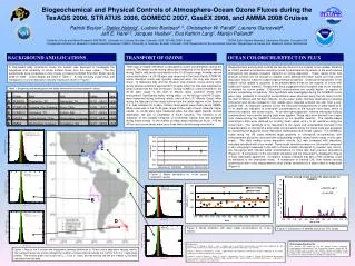
Biogeochemical and Physical Controls of Atmosphere-Ocean Ozone Fluxes during the TexAQS2006, STRATUS 2006, GOMECC 2007, GasEX 2008, and AMMA 2008 Cruises Patrick Boylan1, DetlevHelmig1, Ludovic Bariteau2, 3, Christopher W. Fairall2, Laurens Ganzeveld4, Jeff E. Hare2,3, Jacques Hueber1, Eva Kathrin Lang1,MartijnPallandt4 1Institute of Arctic and Alpine Research (INSTAAR), University of Colorado, Boulder, Colorado, USA; 303-492-2509, E-mail: detlev.helmig@colorado.edu; 2NOAA Earth System Research Laboratory, Boulder, Colorado USA 3Cooperative Institute for Research in Environmental Sciences (CIRES), University of Colorado, Boulder, Colorado, USA;4Department of Environmental Sciences, Wageningen University and Research Centre, Netherlands TRANSPORT OF OZONE BACKGROUND AND LOCATIONS OCEAN COLOR/CHL/EFFECT ON FLUX There was a notable difference in atmospheric ozone concentrations during the cruises. The lowest ozone mixing ratios were measured in the Southern Atlantic during GasEx, with levels consistently in the 15–25 ppbv range. A similar narrow ozone distribution, i.e. 25–35 ppbv, was observed in the South Pacific STRATUS cruise. Elevated ozone was typically observed when the ship was closer to shore. In Galveston Bay and the Houston ship channel, ozone mixing ratios during several occasions approached 100 ppbv when the ship was subjected to urban outflow from the City of Houston. During GOMECC ozone remained in the 20–30 ppbv range in the Gulf of Mexico when southerly winds were encountered. Significantly higher mixing ratios, i.e. 40–60 ppbv and 40-70 ppbv, were measured during northerly winds, and off the U.S. Atlantic Coast, when during the later part of the cruise outflow from the urban regions in the Eastern U.S. was sampled for 6 days. Similar observations were made during AMMA. While ozone was in the 10–30 ppbv range off the coast of South America, higher values, i.e. 40–60 ppbv were measured when the ship sailed towards its final destination, the port of Charleston in South Carolina. This behavior is an indication of the variable influence of continental outflow that was sampled during those cruises. In the outflow of urban areas reaching as far as ~100 km off the coast ozone levels were up to three times above background levels. A ship-based eddy covariance ozone flux system was deployed to investigate the magnitude and variability of ozone surface fluxes over the open ocean. The flux experiments were conducted on five cruises on board the NOAA Ship Ron Brown during 2006 to 2008. Cruise details are listed in Table 1. A map showing cruise track and histograms of ozone deposition velocity results are shown in Figure1. Biogeochemical and physical controls are the key drivers in the oceanic ozone uptake. Fairall et al. (2007) applied a turbulence-chemistry model to parameterize the effects of the wind induced atmosphere and oceanic turbulent transport on ozone deposition. These results show that physical controls are not enough to explain ozone atmosphere-ocean fluxes and that ozone deposition may be linked to ocean biogeochemical properties. Chemical enhancement in the oceanic ozone uptake is assumed to be predominantly driven by the reaction of ozone with iodide and organic material. Researchers have suggested that chlorophyll may be an indicator or reactant for ozone uptake. Chlorophyll concentrations are usually higher in regions of primary productivity or bioactivity. This hypothesis was investigated during the GOMECC cruise when large gradients in chlorophyll concentrations were observed along the US coast in both the Gulf of Mexico and Northern Atlantic. In-situ ocean water chemical observations including chlorophyll and nitrate (needed to infer iodide) were collected onboard the ship from a sub-surface inlet. An important question is how the chlorophyll measurements in water taken at 3-10 m depth are indicative of chlorophyll concentrations at the surface micro-layer, which is where the reaction with ozone occurs. As an alternative approach, inferred chlorophyll surface concentrations from remote sensing data were applied. These data were derived from ocean color measured by the SeaWiFS instrument on the SeaStar satellite. The satellite-based chlorophyll-a data were obtained as monthly mean values at 9 x 9 km resolution along the cruise track. The sensitivity of O3 deposition to the inputs and uncertainties involved in the characterization of chlorophyll-a and iodide concentrations along the cruise track was assessed by comparing the acquired ozone deposition observations with model outputs. The GOMECC cruise along the US coast reflected large gradients in chlorophyll concentrations, with enhancements along the coast and with substantially smaller values farther away on the open ocean. The daily median ozone deposition velocity (Vd) was compared with deposition velocities simulated with a box model. Three model simulations were run: chlorophyll measured in-situ, chlorophyll measured in-situ with a 4 times smaller chlorophyll-O3 reaction rate, and in-situ chlorophyll with inferred iodide concentrations 10 times less than previous simulations (Figure 2). A comparison of the low iodide simulation and the measured Vd displayed in Figure 3 show reasonable agreement. Correlation analysis indicated that 46% of the variability could be attributed to the chlorophyll levels. A comparison of inferred CHL from remote sensing observations with in-situ measurements show similar variability but a slight offset in magnitude (Figure 4). Table 1: Beginning and ending ports and dates covered for the five research cruises. C A Figure 2: Model simulations vs. in-situ ozone deposition results. E B D Figure 3: Model simulation with lower iodide concentrations vs. in-situ results. Figure 4: Comparison of satellite and in-situ CHL results. Acknowledgements: This research was funded by the US National Science Foundation, Interdisciplinary Biocomplexity in the Environment Program, Project No. BE-IDEA 0410058 and by a grant from NOAA’s Climate and Global Change Program, NA07OAR4310168. We thank Joseph Salisbury, University of New Hampshire, for making available the GOMECC chlorophyll data. References: Bariteau, L., D. Helmig, C. Fairall, J. Hare, J. Hueber, and K. Lang (2010), Determination of oceanic ozone deposition by ship-borne eddy covariance flux measurements, Atmospheric Measurement Techniques, 3(2), 442-455. Fairall C, Helmig D, Ganzeveld L & Hare J (2007) Water-side turbulence enhancement of ozone deposition to the ocean. Atmospheric Chemistry and Physics 7: 443-451 Helmig D., Lang E., Bariteau L., Boylan P., Fairall C., Ganzeveld L., Hare J., Hueber J., Pallandt M. Atmosphere-ocean ozone fluxes during the TexAQS 2006, STRATUS 2006, GOMECC 2007, GasEX 2008, and AMMA 2008 cruises. Submitted for publication to J. Geophys. Res. March 2011. Figure 1: Map of the 5 cruises and histograms showing distribution of 10-min ozone deposition velocity results. The numbers above the arrows indicate the number of values that fall outside the -0.25 to 0.5 cm s-1 data range plotted. The vertical green line shows the vd = 0 cm s-1 value, and the vertical red line the median vd that was calculated from the data.