Download
1 / 93
930 likes | 1.16k Views
Extending Expectation Propagation on Graphical Models. Yuan (Alan) Qi Yuanqi@mit.edu. Motivation. Graphical models are widely used in real-world applications, such as human behavior recognition and wireless digital communications. Inference on graphical models: infer hidden variables

E N D
Extending Expectation Propagation on Graphical Models Yuan (Alan) Qi Yuanqi@mit.edu
Motivation • Graphical models are widely used in real-world applications, such as human behavior recognition and wireless digital communications. • Inference on graphical models: infer hidden variables • Previous approaches often sacrifice efficiency for accuracy or sacrifice accuracy for efficiency. > Need methods that better balance the trade-off between accuracy and efficiency. • Learning graphical models : learning model parameters • Overfitting problem: Maximum likelihood approaches >Need efficient Bayesian training methods
Outline • Background: • Graphical models and expectation propagation (EP) • Inference on graphical models • Extending EP on Bayesian dynamic networks • Fixed lag smoothing: wireless signal detection • Different approximation techniques: Poisson tracking • Combining EP with local propagation on loopy graphs • Learning conditional graphical models • Extending EP classification to perform feature selection • Gene expression classification • Training Bayesian conditional random fields • FAQ labeling • Handwritten ink analysis • Conclusions
Outline • Background • 4 kinds of graphical models • Bayesian integration techniques • EP in a nutshell • Inference on graphical models • Learning conditional graphical models • Conclusions
t1 t2 t1 t2 x1 x2 w x1 x2 w x1 x2 x1 x2 y1 y2 y1 y2 Graphical Models INFERENCE LEARNING
Bayesian Integration Techniques (1) • Monte Carlo • Markov Chain Monte Carlo (MCMC), e.g., Hasting algorithm, Gibbs sampler • (Sequential) Importance sampling, e.g., particle filter and smoothers • Quadrature: numerical approximation • Laplace’s method: fitting a Guassian to the mode • Variational method: converting inference to an optimization problem by lower- or upper-bounding techniques.
Bayesian Integration Techniques(2) • Expectation propagation (Minka 01): efficient deterministic approximation techniques.
Expectation Propagation in a Nutshell • Approximate a probability distribution by simpler parametric terms (Minka 2001): • For Bayesian networks: • For Markov networks: • For conditional classification: • For conditional random fields: Each approximation term or lives in an exponential family (such as Gaussian & Multinomial)
EP in a Nutshell (2) • The approximate term minimizes the following KL divergence by moment matching: Where the leave-one-out approximation is
EP in a Nutshell (3) Three key steps: • Deletion Step: approximate the “leave-one-out” predictive posterior for the ithpoint: • Minimizing the following KL divergence by moment matching (Assumed Density filtering): • Inclusion:
Limitations of Plain EP • Batch processing of terms: not online • Can be difficult or expensive to analytically compute ADF step • Can be expensive to compute and maintain a valid approximation distribution q(x), which is coherent under marginalization • Tree-structured q(x): • EP classification degenerates in the presence of noisy features. • Cannot incorporate denominators
Four Extensions on Four Types of Graphical Models • Fixed-lag smoothing and embedding different approximation techniques for dynamic Bayesian networks • Allow a structured approximation to be globally non-coherent, while only maintaining local consistency during inference on loopy graphs. • Combine EP with ARD for classification with noisy features • Extend EP to train conditional random fields with a denominator (partition function)
t1 t2 t1 t2 x1 x2 w x1 x2 w x1 x2 x1 x2 y1 y2 y1 y2 Inference on dynamic Baysian networks
Outline • Background • Inference on graphical models • Extending EP on Bayesian dynamic networks • Fixed lag smoothing: wireless signal detection • Different approximation techniques: Poisson tracking • Combining EP with junction tree algorithm on loopy graphs • Learning conditional graphical models • Conclusions
Object Object Tracking Guess the position of an object given noisy observations
x1 x2 xT y1 y2 yT Bayesian Network e.g. (random walk) want distribution of x’s given y’s
Deterministic Filtering on NonlinearNon-Gaussian Dynamic Models • Extended Kalman filter (EKF): • The process and measurement equations are linearized by a Taylor expansion about the current state estimate. The noise variance in the equations is not changed, i.e. the additional error due to linearization is not modeled. After linearization, the Kalman filter is applied.
Deterministic Filtering on NonlinearNon-Gaussian Dynamic Models • Linear-regression Filter: • The nonlinear/non-Gaussian measurement equation is converted into a linear-Gaussian equation by regressing the observation onto the state (Minka 01). The result is a Kalman lter whose Kalman gain is Cov(state,measurement)Var(measurement) For example, the unscented Kalman filter (Wan and van der Merwe 00), which uses the unscented transformation to measure the state-measurement covariance.
Deterministic Filtering on NonlinearNon-Gaussian Dynamic Models • Assumed-density Filters Choose the Gaussian belief which is closest in KL-divergence to the exact state posterior given previous beliefs. • Mixture of Kalman Filters Pruning the number of Gaussians in the exact posterior to avoid explosion of Guassians.
Sequential Monte Carlo • Particle Filters Using sequential importance sampling with resampling steps. • The proposal distribution is very important • A lot of samples are needed for accurate estimation • EKF- and UKF-Particle Filters. Using EKF or UKF to generate proposal distributions for particle filters
Combining Sequential Monte Carlo withDeterministic Filters • Rao-Blackwellised Particle Filter and Stochastic Mixture of Kalman Filters. • Only draw samples in a subspace which is marginalized over the variables for which we can do exact inference.
Smoothing on Nonlinear Non-GaussianDynamic Models • Particle smoothing • Markov chain Monte Carlo • Extended Kalman smoothing • Variational methods • Expectation propagation
EP Approximation Factorized and Gaussian in x
xt yt Message Interpretation = (forward msg)(observation msg)(backward msg) Forward Message Backward Message Observation Message
Extensions of EP • Instead of batch iterations, use fixed-lag smoothing for online processing. • Instead of assumed density filtering, use any method for approximate filtering. • Examples: EKF, unscented Kalman filter (UKF) Turn any deterministic filtering method into a smoothing method! All methods can be interpreted as finding linear/Gaussian approximations to original terms. • Use quadrature or Monte Carlo for term approximations
y1 yT y2 s1 s2 sT xT x2 x1 Bayesian network for Wireless Signal Detection si: Transmitted signals xi: Channel coefficients for digital wireless communications yi: Received noisy observations
Experimental Results (Chen, Wang, Liu 2000) Signal-Noise-Ratio Signal-Noise-Ratio EP outperforms particle smoothers in efficiency with comparable accuracy.
Extended EP is about than Rao-blackwellised particle smoothers! Computational Complexity • L: Length of fixed-lag smooth window • d: Dimension of the parameter vector • n: Number of EP iterations (Typically, 4 or 5) • M: Number of samples in filtering (Often larger than 500 or 100) • N: Number of samples in smoothing (Larger than 50)
Example: Poisson Tracking • is an integer valued Poisson variate with mean
Accuracy/Efficiency Tradeoff (TIME)
t1 t2 t1 t2 x1 x2 w x1 x2 w x1 x2 x1 x2 y1 y2 y1 y2 Inference on markov networks
Outline • Background • Inference on graphical models • Extending EP on Bayesian dynamic networks • Fixed lag smoothing: wireless signal detection • Different approximation techniques: poisson tracking • Combining EP with junction tree algorithm on loopy graphs • Learning conditional graphical models • Conclusions
X1 X2 X3 X4 X5 X6 X7 X8 X9 X10 X11 X12 X13 X14 X15 X16 Inference on Loopy Graphs Problem: estimate marginal distributions of the variables indexed by the nodes in a loopy graph, e.g., p(xi), i = 1, . . . , 16.
4-node Loopy Graph Joint distribution is product of pairwise potentials for all edges: Want to approximate by a simpler distribution
BP vs. TreeEP projection projection TreeEP BP
Junction Tree Representation p(x) q(x) Junction tree p(x) q(x) Junction tree
Two Kinds of Edges • On-tree edges, e.g., (x1,x4):exactly incorporated into the junction tree • Off-tree edges, e.g., (x1,x2): approximated by projecting them onto the tree structure
KL Minimization • KL minimization moment matching • Match single and pairwise marginals of and
x5 x7 x5 x7 x1 x2 x1 x2 x1 x3 x1 x4 x3 x6 x3 x5 x1 x3 x3 x5 x3 x6 x1 x4 x1 x2 x1 x3 x1 x4 x3 x5 x3 x4 x5 x7 x3 x6 x1 x2 x1 x2 x1 x3 x1 x4 x1 x3 x1 x4 x3 x5 x3 x5 x5 x7 x3 x6 x5 x7 x3 x6 x6 x7 Matching Marginals on Graph (1) Incorporate edge (x3 x4) (2) Incorporate edge (x6 x7)
Drawbacks of Global Propagation by Regular EP • Update all the cliques even when only incorporating one off-tree edge • Computationally expensive • Store each off-tree data message as a whole tree • Require large memory size
Solution: Local Propagation • Allow q(x) be non-coherentduring the iterations. It only needs to be coherent in the end. • Exploit the junction tree representation: only locallypropagate information within the minimal loop (subtree) that is directly connected to the off-tree edge. • Reduce computational complexity • Save memory
x1 x2 x5 x7 x1 x2 x1 x2 x5 x7 x5 x7 x1 x2 x1 x3 x1 x4 x3 x5 x1 x3 x3 x6 x3 x6 x3 x5 x1 x3 x1 x4 x1 x4 x3 x5 x3 x6 x1 x3 x1 x4 x3 x4 x3 x5 x3 x5 x5 x7 x3 x6 x6 x7 (1) Incorporate edge(x3 x4) (2) Propagate evidence On this simple graph, local propagation runs roughly 2 times faster and uses 2 times less memory to store messages than plain EP (3) Incorporate edge (x6 x7)
Tree-EP • Combine EP with junction algorithm • Can perform efficiently over hypertrees and hypernodes
Fully-connected graphs • Results are averaged over 10 graphs with randomly generated potentials • TreeEP performs the same or better than all other methods in both accuracy and efficiency!
t1 t2 t1 t2 x1 x2 w x1 x2 w x1 x2 x1 x2 y1 y2 y1 y2 Learning Conditional Classification Models
Outline • Background • Inference on graphical models • Learning conditional graphical models • Extending EP classification to perform feature selection • Gene expression classification • Training Bayesian conditional random fields • Handwritten ink analysis • Conclusions
Motivation Task 1: Classify high dimensional datasets with many irrelevant features, e.g., normal v.s. cancer microarray data. Task 2: Sparse Bayesian kernel classifiers for fast test performance.
Outline • Background • Bayesian classification model • Automatic relevance determination (ARD) • Risk of Overfitting by optimizing hyperparameters • Predictive ARD by expectation propagation (EP): • Approximate prediction error • EP approximation • Experiments • Conclusions
Bayesian Classification Model Labels: t inputs: X parameters: w Likelihood for the data set: Prior of the classifier w: Where is a cumulative distribution function for a standard Gaussian.
Evidence and Predictive Distribution The evidence, i.e., the marginal likelihood of the hyperparameters : The predictive posterior distribution of the label for a new input :