Download
1 / 24
240 likes | 408 Views
Observation on Parallel Computation of Transitive and Max-closure Problems. Lecture 17. Motivation. TC problem has numerous applications in many areas of computer science. Lack of course-grained algorithms for distributed environments with slow communication.

E N D
Observation on Parallel Computation of Transitive and Max-closure Problems Lecture 17
Motivation • TC problem has numerous applications in many areas of computer science. • Lack of course-grained algorithms for distributed environments with slow communication. • Decreasing the number of dependences in a solution could improve a performance of the algorithm.
What is transitive closure? GENERIC TRANSITIVE CLOSURE PROBLEM (TC) Input:a matrix A with elements from a semiring S= < , > Output:the matrix A*, A*(i,j) is the sum of all simple paths from i to j < , > TC < or , and > boolean closure - TC of a directed graph < MIN, + > all pairs shortest path <MIN, MAX> minimum spanning tree {all(i,j): A(i,j)=A*(i,j)}
Fine–grain and Coarse-grained algorithms for TC problem • Warshall algorithm (1 stage) • Leighton algorithm (2 stages) • Guibas-Kung-Thompson (GKT) algorithm (2 or 3 stages) • Partial Warshall algorithm (2 stages)
X X X Y Y Y Warshall algorithm k k+1 k+2 for k:=1 to n for all 1i,jn parallel do Operation(i, k, j) ---------------------------------- Operation(i, k, j): a(i,j):=a(i,j) a(i,k) a(k,j) ---------------------------------- k k+1 k+2 Warshall algorithm
4 4 4 2 1 1 6 2 4 3 5 2 3 4 4 4
Coarse-Grained computations A11 A24 n A32 n
Actual = Naïve Course Grained Algorithms
Actual = 1 6 2 4 3 5 II I
Course-grained Warshall algorithm Algorithm Blocks-Warshall for k :=1 to N do A(K,K):=A*(K,K) for all 1 I,J N, I K J parallel do Block-Operation(K,K,J) and Block-Operation(I,K,K) for all 1 I,J N parallel do Block-Operation(I,K,J) ---------------------------------------------------------------------- Block-Operation(I, K, J): A(I,J):=A(I,J) A(I,K) A(K,K) A(K,J) ----------------------------------------------------------------------
Implementation of Warshall TC Algorithm k k k k k The implementation in terms of multiplication of submatrices
NEW 1 6 2 4 3 5 II I
Decomposition properties In order to package elementary operations into computationally independent groups we consider the following decomposition properties: • A min-path from i to j is a path whose intermediate nodes have numbers smaller than min (i,j) • A max-path from i to j is a path whose intermediate nodes have numbers smaller than max(i,j)
A’ A B C B’ C’ KGT algorithm KGT algorithm
an initial path 7 a max-path 5 6 3 4 1 2 It is transitive closure closure of the graph An example graph
What is Max-closure problem? • Max-closure problem is a problem of computing all max-paths in a graph • Max-closure is a main ingredient of the TC closure
Max-Closure --> TC Max-to-Transitive performs 1/3 of the total operations Max-closure algorithm Max-closure computation performs 2/3 of total operations The algorithm ”Max-to-Transitive ”reduces TC to matrix multiplication once the Max-Closure is computed
A Fine Grained Parallel Algorithm Algorithm Max-Closure for k :=1 to n do for all 1 i,j n, max(i,j) > k, ij parallel do Operation(i,k,j) Algorithm Max-to-Transitive Input: matrix A, such that Amax = A Output: transitive closure of A For all k n parallel do For all i,j max(i,j) <k, ij Parallel do Operation(i,k,j)
Coarse-grained Max-closure Algorithm Algorithm CG-Max-Closure {Partial Blocks-Warshall} for K:=1 to N do A(K,K):= A*(K,K) for all 1 I,J N, I K J parallel do Block-Operation(K,K,J) and Block-Operation(I,K,K) for all 1 I,J N, max(I,J) > K MIN(I,J) parallel do Block-Operation(I,K,J) -------------------------------------------------------------------------------- Blocks-Operation(I, K, J): A(I,J):=A(I,J) A(I,K) A(K,J)
Implementation of Max-ClosureAlgorithm k k k k k The implementation in terms of multiplication of submatrices
Experimental results ~3.5 h
Increase / Decrease of overall time • While computation time decreases when adding processes the communication time increase => there is an ”ideal” number of processors • All experiments were carried out on cluster of 20 workstations => some processes were running more than one worker-process.
Conclusion • The major advantage of the algorithm is the reduction of communication cost at the expense of small communication cost • This fact makes algorithm useful for systems with slow communication