Quantitative Data Analysis

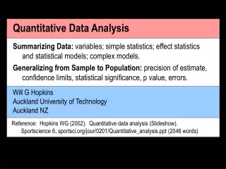
1. Summarizing Data: variables; simple statistics; effect statistics and statistical models; complex models. Generalizing from Sample to Population: precision of estimate, confidence limits, statistical significance, p value, errors. Quantitative Data Analysis Will G HopkinsAuckland University of TechnologyAuckland NZ Reference: Hopkins WG (2002). Quantitative data analysis (Slideshow). Sportscience 6, sportsci.org/jour/0201/Quantitative_analysis.ppt (2046 words)

2. Summarizing Data • Data are a bunch of values of one or more variables. • A variable is something that has different values. • Values can be numbers or names, depending on the variable: • Numeric, e.g. weight • Counting, e.g. number of injuries • Ordinal, e.g. competitive level (values are numbers/names) • Nominal, e.g. sex (values are names • When values are numbers, visualize the distribution of all values in stem and leaf plots or in a frequency histogram. • Can also use normal probability plots to visualize how well the values fit a normal distribution. • When values are names, visualize the frequency of each value with a pie chart or a just a list of values and frequencies.

3. A statistic is a number summarizing a bunch of values. • Simple or univariate statistics summarize values of one variable. • Effect or outcome statistics summarize the relationship between values of two or more variables. • Simple statistics for numeric variables… • Mean: the average • Standard deviation: the typical variation • Standard error of the mean: the typical variation in the mean with repeated sampling • Multiply by (sample size) to convert to standard deviation. • Use these also for counting and ordinal variables. • Use median (middle value or 50th percentile) and quartiles (25th and 75th percentiles) for grossly non-normally distributed data. • Summarize these and other simple statistics visually with box and whisker plots.

4. Y X Model/Test Effect statistics numeric numeric regression slope, intercept, correlation numeric nominal t test, ANOVA mean difference nominal nominal chi-square frequency difference or ratio nominal numeric categorical frequency ratio per… • Simple statistics for nominal variables • Frequencies, proportions, or odds. • Can also use these for ordinal variables. • Effect statistics… • Derived from statistical model (equation) of the form Y (dependent) vs X (predictor or independent). • Depend on type of Y and X . Main ones:

5. body fat(%BM) • Model: numeric vs numerice.g. body fat vs sum of skinfolds • Model or test: linear regression • Effect statistics: • slope and intercept= parameters • correlation coefficient or variance explained (= 100·correlation2)= measures of goodness of fit • Other statistics: • typical or standard error of the estimate= residual error= best measure of validity (with criterion variable on the Y axis) sum skinfolds (mm)

6. Model: numeric vs nominale.g. strength vs sex • Model or test: • t test (2 groups) • 1-way ANOVA (>2 groups) • Effect statistics: • difference between meansexpressed as raw difference, percent difference, or fraction of the root mean square error (Cohen's effect-size statistic) • variance explained or better (variance explained/100)= measures of goodness of fit • Other statistics: • root mean square error= average standard deviation of the two groups strength female male sex

7. Trivial effect: Very large effect: females females males males strength strength • More on expressing the magnitude of the effect • What often matters is the difference between means relative to the standard deviation:

8. Correlations Cohen: 0 0.1 0.3 0.5 Hopkins: 0 0.1 0.3 0.5 0.7 0.9 1 trivial small moderate large very large !!! Effect Sizes Cohen: 0 0.2 0.5 0.8  Hopkins: 0 0.2 0.6 1.2 2.0 4.0 • Fraction or multiple of a standard deviation is known as theeffect-size statistic (or Cohen's "d"). • Cohen suggested thresholds for correlations and effect sizes. • Hopkins agrees with the thresholds for correlations but suggests others for the effect size: • For studies of athletic performance, percent differences or changes in the mean are better than Cohen effect sizes.

9. Model: numeric vs nominal (repeated measures)e.g. strength vs trial • Model or test: • paired t test (2 trials) • repeated-measures ANOVA withone within-subject factor (>2 trials) • Effect statistics: • change in mean expressed as raw change, percent change, or fraction of the pre standard deviation • Other statistics: • within-subject standard deviation (not visible on above plot) = typical error: conveys error of measurement • useful to gauge reliability, individual responses, and magnitude of effects (for measures of athletic performance). strength pre post trial

10. females males • Model: nominal vs nominale.g. sport vs sex • Model or test: • chi-squared test or contingency table • Effect statistics: • Relative frequencies, expressed as a difference in frequencies, ratio of frequencies (relative risk), or ratio of odds (odds ratio) • Relative risk is appropriate for cross-sectional or prospective designs. • risk of having rugby disease for males relative to females is (75/100)/(30/100) = 2.5 • Odds ratio is appropriate for case-control designs. • calculated as (75/25)/(30/70) = 7.0 30% 75% rugby yes rugby no

11. 100 heartdisease(%) • Model: nominal vs numerice.g. heart disease vs age • Model or test: • categorical modeling • Effect statistics: • relative risk or odds ratioper unit of the numeric variable(e.g., 2.3 per decade) • Model: ordinal or counts vs whatever • Can sometimes be analyzed as numeric variables using regression or t tests • Otherwise logistic regression or generalized linear modeling • Complex models • Most reducible to t tests, regression, or relative frequencies. • Example… 0 30 50 70 age (y)

12. drug • Model: controlled trial (numeric vs 2 nominals)e.g. strength vs trial vs group • Model or test: • unpaired t test of change scores (2 trials, 2 groups) • repeated-measures ANOVA withwithin- and between-subject factors (>2 trials or groups) • Note: use line diagram, not bar graph, for repeated measures. • Effect statistics: • difference in change in mean expressed as raw difference, percent difference, or fraction of the pre standard deviation • Other statistics: • standard deviation representing individual responses (derived from within-subject standard deviations in the two groups) strength placebo pre post trial

13. Model: extra predictor variable to "control for something"e.g. heart disease vs physical activity vs age • Can't reduce to anything simpler. • Model or test: • multiple linear regression or analysis of covariance (ANCOVA) • Equivalent to the effect of physical activity with everyone at the same age. • Reduction in the effect of physical activity on disease when age is included implies age is at least partly the reasonormechanism for the effect. • Same analysis gives the effect of age with everyone at same level of physical activity. • Can use special analysis (mixed modeling) to include a mechanism variable in a repeated-measures model. See separate presentation at newstats.org.

14. Problem: some models don't fit uniformly for different subjects • That is, between- or within-subject standard deviations differ between some subjects. • Equivalently, the residuals are non-uniform (have different standard deviations for different subjects). • Determine by examining standard deviations or plots of residuals vs predicteds. • Non-uniformity makes p values and confidence limits wrong. • How to fix… • Use unpaired t test for groups with unequal variances, or… • Try taking log of dependent variable before analyzing, or… • Find some other transformation. As a last resort… • Use rank transformation: convert dependent variable to ranks before analyzing (= non-parametric analysis–same as Wilcoxon, Kruskal-Wallis and other tests).

15. Generalizing from a Sample to a Population • You study a sample to find out about the population. • The value of a statistic for a sample is only an estimate of the true (population) value. • Express precision or uncertainty in true value using 95% confidence limits. • Confidence limits represent likely range of the true value. • They do NOT represent a range of values in different subjects. • There's a 5% chance the true value is outside the 95% confidence interval: the Type 0 error rate. • Interpret the observed value and the confidence limits as clinically or practically beneficial, trivial, or harmful. • Even better, work out the probability that the effect is clinically or practically beneficial/trivial/harmful. See sportsci.org.

16. Statistical significance is an old-fashioned way of generalizing, based on testing whether the true value could be zero or null. • Assume the null hypothesis: that the true value is zero (null). • If your observed value falls in a region of extreme values that would occur only 5% of the time, you reject the null hypothesis. • That is, you decide that the true value is unlikely to be zero; you can state that the result is statistically significant at the 5% level. • If the observed value does not fall in the 5% unlikely region, most people mistakenly accept the null hypothesis: they conclude that the true value is zero or null! • The p value helps you decide whether your result falls in the unlikely region. • If p<0.05, your result is in the unlikely region.

17. One meaning of the p value: the probability of a more extreme observed value (positive or negative) when true value is zero. • Better meaning of the p value: if you observe a positive effect, 1 - p/2is the chance the true value is positive, and p/2 is the chance the true value is negative. Ditto for a negative effect. • Example: you observe a 1.5% enhancement of performance (p=0.08). Therefore there is a 96% chance that the true effect is any "enhancement" and a 4% chance that the true effect is any "impairment". • This interpretation does not take into account trivial enhancements and impairments. • Therefore, if you must use p values, show exact values, not p<0.05 or p>0.05. • Meta-analysts also need the exact p value (or confidence limits).

18. If the true value is zero, there's a 5% chance of getting statistical significance: the Type I error rate, or rate of false positives or false alarms. • There's also a chance that the smallest worthwhile true value will produce an observed value that is not statistically significant: the Type II error rate, or rate of false negatives or failed alarms. • In the old-fashioned approach to research design, you are supposed to have enough subjects to make a Type II error rate of 20%: that is, your study is supposed to have a power of 80% to detect the smallest worthwhile effect. • If you look at lots of effects in a study, there's an increased chance being wrong about at least one of them. • Old-fashioned statisticians like to control this inflation of the Type I error rate within an ANOVA to make sure the increased chance is kept to 5%. This approach is misguided.

19. High reliability p = 0.003 Low reliability p = 0.2 Mean ± SEM in both cases what- ever pre post pre post pre post • The standard error of the mean (typical variation in the mean from sample to sample) can convey statistical significance. • Non-overlap of the error bars of two groups implies a statistically significant difference, but only for groups of equal size (e.g. males vs females). • In particular, non-overlap does NOT convey statistical significance in experiments:

20. In summary • If you must use statistical significance, show exactp values. • Better still, show confidence limits instead. • NEVER show the standard error of the mean! • Show the usual between-subject standard deviation to convey the spread between subjects. • In population studies, this standard deviation helps convey magnitude of differences or changes in the mean. • In interventions, show also the within-subject standard deviation (the typical error) to convey precision of measurement. • In athlete studies, this standard deviation helps convey magnitude of differences or changes in mean performance.