DATA TYPES AND QUANTITATIVE DATA ANALYSIS
DATA TYPES AND QUANTITATIVE DATA ANALYSIS. PRESENTED TO THIRD-TRIMESTER YEAR 1. DATA. Information expressed qualitatively or quantitatively Data are measurements of characteristics Measurements are functions that assign values in quantitative or quantitative form

DATA TYPES AND QUANTITATIVE DATA ANALYSIS
E N D
Presentation Transcript
DATA TYPES AND QUANTITATIVE DATA ANALYSIS PRESENTED TO THIRD-TRIMESTER YEAR 1
DATA • Information expressed qualitatively or quantitatively • Data are measurements of characteristics • Measurements are functions that assign values in quantitative or quantitative form • Characteristics are referred to as variables Eg. Height, weight, sex, tribe, etc
VARIABLES AND DATA TYPES • Variable as characterization of event • Classification of Variables • Qualitative: usually categorical; values/members fall into one of a set of mutually exclusive & collectively exhaustive classes. eg. Sex, crop variety, animal breed, source of water, type of house • Quantitative: numeric values possessing an inherent order. • Discrete: eg. # of children/farmers/animals, etc • Continuous: height, weight, distance, etc • Random and Fixed
Data Types • Scales of measurements • Nominal • Ordinal • Interval • Ratio Levels of measurement distinguished on the basis of the following criteria: • Magnitude or size; Direction • Distance or interval; Origin • Equality of points; Ratios of intervals; Ratio of points
NOMINAL DATA • Example: Sex (Gender) coded M,F or 0,1 • ‘Numbers’ simply identify, classify, categorize or distinguish. • The score has nosize or magnitude • Score has equality because two subjects are similar (equal) if they have same number • Weakest level of measurement; poor • ArithmeticoperationsCANNOT be performed on nominal data types
ORDINAL DATA • Associated with qualitative random variables • Generated from ranked responses (or from a counting process). • Have properties of nominal-data, in addition to DIRECTION • Numeric or non-numeric • Next to nominal in terms of weakness • Arithmeticoperations must be avoided • Egs: knowledge (low, average, high), socio-economic status, attitude, opinion (like, dislike, strongly dislike), etc.
INTERVAL and RATIO INTERVAL • Numeric, have magnitude or size, direction, distance or interval, and origin • Interval scale has no absolute 0 that is NOT independent of system of measurement [0oC not same temperature as 0oF] • Eg. Temperature in degrees Fahrenheit or Celsius RATIO • Weight of cassava in kilogram or pounds weight • Numeric, have magnitude or size, direction, distance or interval, and origin • Absolute origin exists and not system dependent All arithmetic operations can be performed on such data types
DATA COLLECTION PROCESSES • Processes include (not mutually exclusive) • Routine Records; • Survey Data; • Experimental data;
ROUTINE (MONITORING) DATA • Data periodically recorded essentially for administrative use of the establishment and for studying trends or patterns. • Examples – medical records, meteorological data • Some statistical analysis of data possible on description and prescription • Cheap data, and planning could be haphazard
EXPERIMENTAL DATA • Treatments are the investigated factors of variation • Treatments are controlled by the designer • Treatment levels may be fixed, random, qualitative, quantitative • Comparative experimental data require inductive analysis • Emphasis on inference including estimation of effects and test of hypotheses.
SURVEY DATA COLLECTION • Information on characteristics, opinions, attitudes, tendencies, activities or operations of the individual units of the population • Based on a small set of the population • Can be planned; preference for random surveys • Researcher or investigator has no (or must not exercise) control over the respondent or data
Which procedure to use? • Depends on study objectives • All 3 procedures are possible while in the community • Monitoring and Survey procedures will be most used during the first year. • We discuss SURVEY further
SAMPLING (SURVEY) METHODS • Ensure units of population have same chance of being in the sample. Sampling Types • Probability sampling - the selection of sampling units is according to a probability (random & non-random) scheme. • Non-probability sampling - selection of samples not objectively made, but influenced a great deal by the sampler. Example – haphazard and use of volunteers • Preference is for probability sampling, but situation may determine otherwise
SYSTEMATIC SAMPLING Procedure • Sampling units are selected according to a pre-determined pattern. • For instance, given a sampling intensity of 10% from a population of 100 numbered trees or units (strips etc) might require your observing every 1 out of 10 trees (units, strips) in an ordered manner or sequence
Selection in Systematic Procedure • E.g. if by some process, random or non-random, the 3rd tree (unit or strip) is selected first, then the 13th, 23rd, 33rd, 43rd,..., 93rd trees (unit, strips) will accordingly be selected. Strictly, this type of selection as illustrated with the population of 100 trees (units) involves only one sample. • Improve by selecting 1st unit randomly from 1 to 10, or 1 to 100, and by MULTIPLE random starts
Applications of Systematic Sampling _ Population is unknown _ Baseline studies on spatial distribution patterns of population _ Baseline studies on extent/distribution of pests, pathogens, etc. _ Mapping purposes _ Regeneration studies
Advantages of Systematic Sampling _ Easy to set-up _ Relative speed in data collection _ Total coverage of population assured _ Good base for future designs, as position of characters can easily be mapped (with known coordinates) _ Demarcation of units not necessary, as sampling units are defined by first unit.
Disadvantages of Systematic Sampling • With only one random observation, sampling error not valid • Unknown trend(s) in population can influence results adversely [Examples: topography, season of sampling interval]
Avoiding the disadvantages • The first major disadvantage on sampling error can be rectified by introducing several multiple random starts through stratification of the population • The second problem of trend is more difficult but simply relates to the choice of the sampling interval.
Simple/Unrestricted Random Sampling • Unlike the systematic sampling, sampling units need not be equally spaced. • We shall define this as that sampling procedure which ensures equal probability for all samples of the same size (without any restriction imposed on the selection process).
Illustration of SRS • Given a pop. Size of N from which a sample of size n will be drawn, the number of possible ways of obtaining the sample is • Supposing a population is known to have 5 units, and a sample size of 3 is required. • From this population of 5 units, there are 10 possible ways of obtaining a sample of size 3. [The formula is 5C3= 5!/{(5-3)! 3!} = 10]. • Each of these combinations is unique and has the same chance (1/10) of being selected. • Thus SRS is a random sampling procedure where each sample of size n has the same probability of selection.
SRS selection process • (i) Select randomly one 'sample combination' from the number 1 to 10 (as there are 10 possible combinations). • (ii) Use the table of random numbers to select 3 numbers from 1 to 5 or select three numbers from a 'hat' containing all the five numbers. This option seems easier and more practicable than (i).
Summary - SRS • Application: Applied when the population is known to be homogeneous. Procedure is suitable for units defined by plot sizes. • Advantage: Easy to apply, though not as easy as the systematic procedure. • Disadvantage: Requires knowledge of all the units in the population (construction of the frame is necessary)
STRATIFIED RANDOM SAMPLING • Requires dividing the population into non-overlapping homogeneous units, which we are called STRATA. • SRS is then applied to each stratum, hence stratified random sampling (STRS). • Examples of strata types or criteria are ages of plantation, species types, aspect, topography/ altitude, farm types, habitat • Dividing the population into such homogeneous units usually leads to better estimates of the desired population parameters.
Where/when to apply Stratified RS • Very suitable for heterogeneous areas (or units) that can be identified and classified into homogeneous entities. • Supplementary information, e.g. rem sensing aerial photographs, useful for stratification. • Choice of strata should ensure variation between units within strata is less than the variation between strata.
Advantages/Disadvantages of STRS Advantages • Estimates are more precise • Separate estimates and inferences for strata are possible Disadvantages • Sample size depends on type of allocation to be used • Sampling likely to be efficient in some strata than others • Errors in strata classification affect overall estimate • Frame construction for each stratum is required.
Allocation of units (n) to strata • Equal allocation - Equal (same) number of units are collected from each stratum. • Proportional allocation - The number of units per strata is proportional to the size of the strata.
ANALYSING QUALITATIVE DATA • Qualitative data are essentially labels of a categorical variable • Statistical Analyses involve totals, percentages and conversion to pie-charts and bar charts (bar-graphs). • Sophisticated analyses include categorical modelling
You can have multiple bar graphs (i.e, can have more than one variable illustrated on a bar chart. Example is given below:
Contingency Table This involves count summaries for 2 or more categories placed in row-column format: Example of a 2 by 3 contingency table: Assess association between Gender & Group
ANALYSING QUANTITATIVE DATA • Basic analyses involve determining the CENTRE and SPREAD of data. • Inferential, probability and non-probability based
Measuring Centre Statistics include • MODE (most frequently occurring observation) • MEDIAN (observation lying at the centre of an ordered data) – best for INCOME data • MEAN (a sufficient, consistent, unbiased statistic, utilising ALL observations)
EXAMPLE • Consider that we selected RANDOMLY 10 houses out of 50, and observed the number of school-aged children who do not go to school as follows: 1 2 4 4 1 1 6 0 5 2 Find MEDIAN, MODE, MEAN
MODE: 1 as it appeared most often (most households have at least 1 child of school-going age not in school) • MEDIAN: Centremost observation after ordering data lies between the 4th and 5th data, i.e., between 2 and 2 (= 352) 0 1 1 1 2 2 4 4 5 6 Interpretation: 50% of the sampled population have up to 2 children of school-going age not in school) • MEAN: We use the arithmetic mean = sum of data divided by no. of observations, = (0+1+1+1+ 2+2+4+4+5+6)/10=2.6
Measuring Spread Statistics include • MINIMUM, MAXIMUM (ie EXTREME data) • RANGE (a single statistic calculated as MAXIMUM minus MINIMUM value) • MEAN of the sum of the ABSOLUTE DEVIATION • STANDARD DEVIATION (SD, but use the divisor n-1, not n as in most calculators). • STANDARD ERROR
EXAMPLE • Consider that we selected RANDOMLY 10 houses out of 50, and observed the number of school-aged children who do not go to school as follows: 1 2 4 4 1 1 6 0 5 2 Find STANDARD DEVIATION, STANDARD ERROR and CONFIDENCE LIMITS
CALCULATING SPREAD: STANDARD DEVIATION Standard Deviation: = 2.01 Approximate SD = = (6-0)/4 = 1.5 (valid if sample is large and distribution is normal)
Sampling fraction (f) and Finite Population Correction Factor (fpc) • Sampling fraction= f = n/N = 10/50 = 0.20 (represents the proportion of the population that is sampled, i.e. observed) • If f < 0.05, fpc is ignored. In our case, f > 0.5 (indeed equals 0.20), fpc must be calculated and used for the sampling errorcomputation fpc = (N-n)/N = 1– n/N = 1- 0.20 = 0.80
Confidence (Fiducial) Limits • Given a level of significance, 5%, can obtain a 95% confidence limit on the mean number of non-school going children by multiplying SE by 1.96, that is: P(2.6-1.96*0.57 < true number < 2.6+1.96*0.57) =1-0.05= 0.95 P(1.5 < true number per household < 3.7) = 0.95 • Interpretation: 95% certain that true number of children in community who are of school-age but at home is between 1.5 (1) and 3.7 (4). OR can conclude (after multiplying by the total 50 households • 75 to 185 school-aged children in the community are not in school
Combining Spread and Centre BOX PLOT HISTOGRAM
Further Analysis of Quantitative Data • Histograms give idea of the distribution of the data; very useful for quantitative data • An excellent alternative to histogram is the stem-leaf diagram. • Measures of association – correlation analysis, dependence (cause-effect) relations (regression procedures) – 2006/2007
DATA ANALYSIS IS ENDLESS!!! • ENJOY YOUR TIME DURING TTFPP • END • KS Nokoe, PT Birteeb, IK Addai, M Agbolosu, L Kyei,