Modeling High-Level Structures in Low-Level Language Processors
270 likes | 294 Views
Learn how to represent high-level computational structures in low-level memory, including data representation, expression evaluation, stack allocation, and routines implementation.

Modeling High-Level Structures in Low-Level Language Processors
E N D
Presentation Transcript
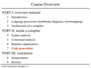
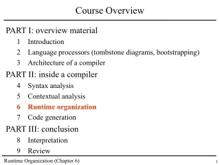
Course Overview PART I: overview material 1 Introduction 2 Language processors (tombstone diagrams, bootstrapping) 3Architecture of a compiler PART II: inside a compiler 4 Syntax analysis 5 Contextual analysis 6Runtime organization 7 Code generation PART III: conclusion • Interpretation 9 Review
What This Chapter is About A compiler translates a program from a high-level language into an equivalent program in a low-level language. The low-level program must be equivalent to the high-level program. => High-level concepts must be modeled in terms of the low-level machine. This chapter is not about the compilation process itself, but about the way we represent high-level structures in terms of a typical low-level machine’s memory architecture and machine instructions. => We need to know this before we can talk about code generation.
What This Chapter is About How to model high-level computational structures and data structures in terms of low-level memory and machine instructions. High-levelProgram Expressions Records Procedures Methods Arrays Variables Objects How to model ? Low-level Language Processor Registers Bits and Bytes Machine Stack Machine Instructions
What This Chapter is About • Data Representation: how to represent values of the source language on the target machine. • Expression Evaluation: How to organize computing the values of expressions (taking care of intermediate results) • Stack Storage Allocation: How to organize storage for variables (considering lifetimes of global and local variables) • Routines: How to implement procedures, functions (and how to pass their parameters and return values) • Heap Storage Allocation: How to organize storage for variables (considering lifetimes of heap variables) • Object Orientation: Runtime organization for OO languages (how to handle classes, objects, methods)
Data Representation • Data Representation: how to represent values of the source language on the target machine. High level data structures Low level memory model word 0: 00..10 Records 1: 01..00 word 2: ... Arrays ? 3: Strings Integer Char … Note: addressing schema and size of “memory units” may vary
Data Representation Important properties of a representation schema: • non-confusion: different values of a given type should have different representations • uniqueness: Each value should always have the same representation. • These properties are very desirable (why?), but in practice they are not always satisfied: • Example: • confusion: approximated floating point numbers. • non-uniqueness: one’s complement representation of integers.
Data Representation Important issues in data representation: • constant-size representation: The representation of all values of a given type should occupy the same amount of space. • direct versus indirect representation Indirect representation of a value x Direct representation of a value x x bit pattern • x bit pattern pointer Q: What reasons could there be for choosing indirect representations?
Indirect Representation Q: What reasons could there be for choosing indirect representations? To make the representation “constant size” even if representation requires different amounts of memory for different values. • small x bit pattern Both are represented by pointers =>Same size • large x bit pattern
Indirect versus Direct The choice between indirect and direct representation is a key decision for a language designer/implementer. • Direct representations are often preferable for efficiency: • More efficient access (no need to follow pointers) • More efficient storage (e.g. stack rather than heap allocation) • For types with widely varying size of representation it is almost a must to use indirect representation (see previous slide) Languages like Pascal, C, C++ try to use direct representation wherever possible. Languages like Scheme, ML use mostly indirect representation everywhere (because of higher order functions) Java: primitive types direct, “reference types” (objects) indirect.
Data Representation • We now survey representation of the more common data types found in programming languages, assuming direct representations wherever possible. • We will discuss representation of values of: • Primitive Types • Record Types • Disjoint Union Types • Static and Dynamic Array Types • Recursive Types • We will use the following notations (if T is a type): • #[T]The cardinality of the type (i.e. the number of possible different values) • size[T] The size of the representation (in number of bits/bytes)
Data Representation: Primitive Types What is a primitive type? The primitive types of a programming language are those types that cannot be decomposed into simpler types. For example integer, boolean, char, etc. Type: boolean Has two values true and false => #[boolean] = 2 => size[boolean] ≥ 1 bit Possible Representations 1bit byte(option 1) byte(option2) 0 00000000 00000000 1 00000001 11111111 Value false true Note: In general, if #[T] = n then size[T] ≥ log2 n bits
Data Representation: Primitive Types Type: integer Fixed size representation, usually dependent (i.e. chosen based on) what is efficiently supported by target machine. Typically uses one word (16 bits, 32 bits, or 64 bits) of storage. size[integer] = word (= 16 bits) => # [integer] ≤ 216 = 65536 Modern processors use two’s complement representation of integers Multiply by -(215) Multiply by 2n n = position from right 1 0 0 0 0 1 0 0 1 0 0 1 0 1 0 1 Value = -1*215 +0*214 +…+0*23+1*22 +1*21 +1*20 Q: What range of values can be represented with 16 bits?
Data Representation: Primitive Types Example: Primitive types in TAM (Triangle Abstract Machine) Type Boolean Char Integer Representation 00...00 and 00...01 Unicode Two’s complement Size 1 word 1 word 1 word Example: A (possible) representation of primitive types on a Pentium Type Boolean Char Integer Representation 00...00 and 11..11 ASCII Two’s complement Size 1 byte 1 byte 1 word
Data Representation: Composite Types • Composite types are types which are not “atomic”, but which are constructed from more primitive types. • Records (called structs in C and classes in C++) • Aggregates of several values of possibly several different types • Arrays • Aggregates of several values of the same type • Disjoint Union Types • Disjoint unions are the “dual” of records. They can have values of several different types, but not more than one at the same time.
Data Representation: Records Example: Triangle Records type Date = record y : Integer, m : Integer, d : Integer end; type Details = record female : Boolean, dob : Date, status : Char end; var today: Date; var my: Details
Data Representation: Records Example: Triangle Record Representation false my.female today.y my.dob.y 2004 1970 3 5 today.m my.dob my.dob.m 2 17 today.d my.dob.d ‘u’ my.status … 1 word:
Data Representation: Records Records occur in some form or other in most programming languages: Ada, Pascal, Triangle (here they are actually called records) C, C++ (here they are called structs) The usual representation of a record type is just the concatenation of individual representations of each of its component types. value of type T1 type T = record I1: T1; I2: T2; ... In: Tn; end; var r: T; r.I1 r.I2 value of type T2 r.In value of type Tn
Data Representation: Records Q: How much space does a record take? And how to access record elements? Example: size[Date] = 3*size[integer]= 3 words address[today.y] = address[today]+0 address[today.m] = address[today]+1 address[today.d] = address[today]+2 address[my.dob.m] = address[my.dob]+1 = address[my]+2 Note: these formulas assume that addresses are indexes of words (not bytes) in memory (otherwise multiply these offsets by 2 or 4)
Data Representation: Records • Problem: Real machines: • Don’t address words • Have alignment concerns • Example: C/C++ on the x86 architecture • size[boolean] = 1 byte • size[char] = 1 byte • size[int] = 4 bytes • Alignment: all data must be laid out on “natural” boundaries • Not for correctness, but for performance
f y y y y m m m m d d d d s ? ? ? y y y y m m m m d d d d s ? ? ? Alignment example struct Date { int y, m, d; }; struct Details { bool female; Date dob; char status; }; f
Data Representation: Disjoint Unions What are disjoint unions? Like a record, has elements which are of different types. But the elements never exist at the same time. A “type tag” determines which of the elements is currently valid. Example: Pascal variant records type Number = record case discrete: Boolean of true: (i: Integer); false: (r: Real) end; var num: Number Mathematically we write disjoint union types as: T = T1 | … | Tn
Data Representation: Disjoint Unions Example: Pascal variant records representation type Number = record case discrete: Boolean of true: (i: Integer); false: (r: Real) end; var num: Number num.discrete num.discrete true false 3.14 15 num.i num.r unused Assuming size[Integer]=size[Boolean]=1 and size[Real]=2, then size[Number] = size[Boolean] + MAX(size[Integer], size[Real]) = 1 + MAX(1, 2) = 3
Data Representation: Disjoint Unions type T = record case Itag: Ttagof v1: (I1: T1); v2: (I2: T2); ... vn: (In: Tn); end; var u: T size[T] = size[Ttag] + MAX(size[T1], ..., size[Tn]) address[u.Itag ] = address[u] address[u.I1] = address[u]+size[Ttag] ... address[u.In] = address[u]+size[Ttag] u.Itag v1 u.Itag v2 u.Itag vn u.I1 type T1 u.I2 type T2 u.In type Tn or … or or
Arrays • An array is a composite data type; an array value consists of multiple values of the same type. Arrays are in some sense like records, except that their elements all have the same type. • The elements of arrays are typically indexed using an integer value (In some languages such as for example Pascal, also other “ordinal” types can be used for indexing arrays). • Two kinds of arrays (with different runtime representation schemas): • static arrays: their size (number of elements) is known at compile time. • dynamic arrays: their size can not be known at compile time because the number of elements may vary at run-time. Q: Which are the “cheapest” arrays? Why?
names[0][0] ‘J’ names[0][1] ‘o’ names[0][2] ‘h’ Name names[0][3] ‘n’ names[0][4] ‘ ’ names[0][5] ‘ ’ names[1][0] ‘S’ names[1][1] ‘o’ names[1][2] ‘p’ Name names[1][3] ‘h’ names[1][4] ‘i’ names[1][5] ‘a’ Static Arrays Example: type Name = array 6 of Char; var me: Name; var names: array 2 of Name me[0] ‘K’ me[1] ‘r’ me[2] ‘i’ me[3] ‘s’ me[4] ‘ ’ me[5] ‘ ’
code[0].c ‘K’ Coding code[0].n 5 code[1].c ‘i’ Coding code[1].n 22 code[2].c ‘d’ Coding code[2].n 4 Static Arrays Example: • type Coding = record • Char c, Integer n • end • var code: array 3 of Coding
Static Arrays typeT = arraynofTE; var a : T; a[0] size[T] = n * size[TE] address[a[0]] = address[a] address[a[1]] = address[a]+size[TE] address[a[2]] = address[a]+2*size[TE] … address[a[k]] = address[a]+k*size[TE] … a[1] a[2] a[n-1]