Undirected Graphical Models

1. Undirected Graphical Models Raul QueirozFeitosa

2. Pros and Cons Advantages of UGMs over DGMs • UGMs are more natural for some domains (e.g. context-dependent entities) Advantages of DGMs over UGMs • Parameters of DGMs are more interpretable than of UGMs • Parameter estimation of UGMs computationally more expensive than of DGMs Undirected Graphical Models

3. Conditional Independence in UGM Check if Procedure: remove all nodes in C with their links. If there is no path connecting any node in A to any node in B, the conditional independence holds. A B C Introduction to Graphical Models

4. UGM vs. DGM Do all probability distributions can be perfectly mapped by either UGMs and/or DGMs? DGM UGM all distributions over a given set of variables Undirected Graphical Models

5. UGM vs. DGM Examples of distributions that can be represented either by an UGM or a DGM: C A A B impossible to represent the same conditional independence properties D B C ? Undirected Graphical Models

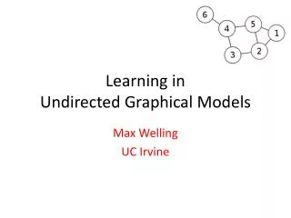
6. Clique Clique: any set of fully connected nodes Maximal clique: a clique such that it is not possible to include any other node from the graph without it ceasing to be a clique. y2 y1 y3 y4 Undirected Graphical Models

7. Site A site represents a point or a region in the Euclidean space such as an image pixel or an image patch. regular irregular Undirected Graphical Models

8. Label A countable set of labels , where • nis the number of sites, • , • is the number of classes, sky field Undirected Graphical Models

9. Neighborhood System Examples of neighborhood systems for a regular set of sites : 4 - Neighborhood 8 - Neighborhood Undirected Graphical Models

10. Markov Random Field Let be the labels at an input image, where corresponds to the ith site, are the set of ineighbors, and is the set of image sites. Definition: is said to be a Markov random field on w.r.t. a neighborhood system , iff the following two conditions hold for all (positivity) (Markovianity) Undirected Graphical Models

11. Gibbs Distribution A set of random variables has a Gibbs distribution on w.r.t. iff where • is the set of all maximal cliques, • are non negative functions • >0 is the energy • is a normalizing constant called partition function. the lower the higher associated with the variables in clique , Undirected Graphical Models

12. Hammersley-Clifford Theorem is a Markov random field on w.r.t. a neighborhood system , ifffollows the Gibbs distribution on w.r.t. a neighborhood system . Undirected Graphical Models

13. Gibbs Random Field Example: from the graph below one can write Pairwise MRF: for simplicity it may be restricted to edges rather than to maximal cliques (henceforth): y3 y5 y1 y4 y2 ! … Undirected Graphical Models

14. MAP-MRF framework In the MRF framework, the posterior over the labels the corresponding set of observed data is expressed using the Bayes’ rule as, where the prior over the labels is modeled as a MRF. Usually, for tractability, the likelihood model, is assumed to have the factorized form ! likelihood ofobservationat site i for class Undirected Graphical Models

15. Pairwise MRF image model Consequently, the posterior takes the form Inference : the classification outcome is given by homogeneous MRF likelihood given by some generative classifier Undirected Graphical Models

16. Pairwise MRF image model Consequently, the posterior takes the form example of a homogeneous MRF Inference : the classification outcome is given by likelihood generative classifier homogeneous MRF Undirected Graphical Models

17. Problems with MAP-MRF framework • The assumption is too restrictive for several natural image analysis applications! • The label interaction does not depend on the data . We may want to “turn-off” label smoothing between two adjacent nodes if there is a discontinuity in image intensity. • To model the posterior we have first to model the likelihood. Undirected Graphical Models

18. Conditional Random Field CRF models the posteriorprobability directly as an RF without modeling the prior and likelihood individually. Association Potential or unaries Interaction Potential or binaries Undirected Graphical Models

19. Conditional Random Field CRF models the posteriorprobability directly as an RF without modeling the prior and likelihood individually. and are features computed upon the observation x. Undirected Graphical Models

20. Conditional Random Field CRF models the posteriorprobability directly as an RF without modeling the prior and likelihood individually. local posterior given by some discriminative classifier Homogeneous CRF Undirected Graphical Models

21. MRF vs CRF MRF: CRF: • Association potentials are likelihoods in MRF and local posteriors in CRF. • Association potential is (might be) a function of local data in MRF and of all data in CRF. • Interaction potential is (might be) a function of labels only in MRF and also of data in CRF. Undirected Graphical Models

22. Example of Interaction Potential Contrast sensitive Potts model: “turns off” smoothing at data discontinuities, e.g., whereby discontinuity is given by Undirected Graphical Models

23. MRF/CRF representation A pairwise MRF/CRF model over a 4 neighborhood regular grid consists of: • Node structure (links) • Node potentials (unaries) M dimensional vectors • Edge potentials (binaries) M×M matrices 1 7 4 2 8 5 3 9 6 Undirected Graphical Models

24. MRF/CRF training • Unaries are trained in a supervised way • Binaries of our examples, i.e., parameter is estimated by cross-validation. • In some cases binaries’ training also follows a supervised approach. Undirected Graphical Models

25. Inference It is about computing • For a grid containing a × b nodes, which may belong to M classes, the number of possibilities is equal to • Exact solution is only feasible for few particular problems. • Efficient approximate algorithms are available. • To further reduce complexity superpixels instead of pixels are used. Undirected Graphical Models

26. Multitemporal CRF

27. Multitemporal CRF row column epoch

28. Multitemporal CRF row column epoch

29. Multitemporal CRF row column epoch

30. Multitemporal CRF row column epoch

31. MarkovAssumption Each site/node is only influenced by its neighbors as defined by the edges that emerge from it. Far away nodes do influence the class on that site/node but indirectly though intermediate edges and nodes. 31

32. Multitemporal CRF hereafter where • - association potential relative to epoch • - spatial interaction potential relative to epoch • - temporal interaction potential relative to epoch • / set of spatial/temporal neighbors of site Solution: Undirected Graphical Models

33. Association Potential

34. Spatial Interaction Potential  classat site j 1 2 M   classat site i

35. Temporal Interaction Potential In manyapplicationstheemporalinteraction ignores anydependenceontheobservations.

36. Temporal Interaction Potential Transition Matrix: notundirected classat site k  1 2 M   classat site i

37. Temporal Interaction Potential Joint Probability Matrix: classat site k  1 2 M   classat site i k

38. Temporal Interaction Potential Just set 1/0 for possible/impossible: classat site k  1 2 M   classat site i

39. References Books and Papers • Christopher M. Bishop, Patter Recognition and Machine Learning, Springer, 2006. Chapter 8. • Daphne Koller & Nir Friedman, Probabilistic Graphical Models, MIT Press, 2009. Chapter 3. • Kevin P. Murphy, Machine Learning – A Probabilistic Approach, MIT Press, 2012, Chapter 19. • Stan Z. Li, Markov Random Field Modeling in Image Analysis, 3rd Ed., Springer, 2010. Chapter 2. • Kumar, S., Hebert, M., Discriminative Random Fields, International Journal of Computer Vision, vol. 68(2), 2006, pp. 179-202. Available at <http://repository.cmu.edu/cgi/viewcontent.cgi?article=1360&context=robotics> Directed Graphical Models

40. References Online lectures • Graphical Models 2 – Christopher Bishop • Graphical Models 3 – Christopher Bishop. • Probabilistic Graphical Models - Daphne Koller MATLAB Library • Schimidt, M., UGM: Matlab code for undirected graphical models, Available athttp://www.cs.ubc.ca/~schmidtm/Software/UGM.html Directed Graphical Models

41. Undirected Graphical Models END Undirected Graphical Models