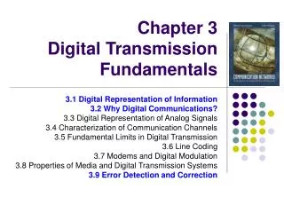
Digital transmission fundamentals (chap.3 & 4)

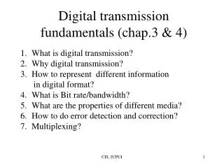
1. Digital transmission fundamentals (chap.3 & 4) • What is digital transmission? • Why digital transmission? • How to represent different information • in digital format? • What is Bit rate/bandwidth? • What are the properties of different media? • How to do error detection and correction? • Multiplexing? CIS, IUPUI

2. What is digital transmission? • Analog transmission • Continuous waveform • Digital representation and transmission • Discrete binary sequence/pulses • 1: a rectangular pulse of amplitude 1 and of duration 0.125 milliseconds • 0: a rectangular pulse of amplitude -1 and of duration of 0.125 milliseconds. CIS, IUPUI

3. CIS, IUPUI Figure 3.13

4. 1 0 1 0 1 0 1 0 (a) . . . . . . t 1 ms 1 1 1 1 0 0 0 0 (b) . . . . . . t 1 ms CIS, IUPUI Figure 3.14

5. Analog Digital ? --PCM • Analog signal such as voice/music: • continuous waveform, i.e, variations in air pressure. • Bandwidth: a measure of how fast the signal varies, i.e., cycles/second, or Hertz. • Two stages: • Sampling: for bandwidth W, minimum sampling rate is 2W. • Quantizing: how many levels to represent a sample. • Example: W=4 kHz, sampling rate=8K samples/second. Sample period is T=1/8000=125 microseconds. Suppose 8 bits/sample (256 levels), then PCM bit rate is 8000*8=64 kbps. CIS, IUPUI

6. (a) 7D/2 5D/2 3D/2 D/2 -D/2 -3D/2 -5D/2 -7D/2 7D/2 (b) 5D/2 3D/2 D/2 -D/2 -3D/2 -5D/2 -7D/2 CIS, IUPUI Figure 3.2

7. Why digital? • For analog: • output should reproduce the input exactly. No distortion. • Repeater amplifies noise, difficult task. • Too much repeaters may make noise too large, so limited distance • Cost is high. • Basic voice/telephone service. • For digital: • Not exact, as long as can distinguish 1 or o. • Digital regenerator generates pure digital numbers, easy. • No limitation on digital regenerators, no distance limitation. • Cost is low. • More other services, easily multiplexing, more functions. CIS, IUPUI

8. Received Sent (a) Analog transmission: all details must be reproduced accurately • e.g. AM, FM, TV transmission (b) Digital transmission: only discrete levels need to be reproduced Received Sent • e.g digital telephone, CD Audio CIS, IUPUI Figure 3.6

9. Transmission segment Destination Source Repeater Repeater CIS, IUPUI Figure 3.7

10. Recovered signal + residual noise Attenuated & distorted signal + noise Amp. Equalizer Repeater CIS, IUPUI Figure 3.8

11. Decision Circuit. & Signal Regenerator Amplifier Equalizer Timing Recovery Distorted Digital signal is easy to restore by regenerator. CIS, IUPUI Figure 3.9

12. Digital representations for different information • Text: ASCII • Scanned WB documents: • A4 paper, 200 X 100 pixels/inch. 256KB. • Color pictures/images: • 8 X 10 inch photo, 400 X400 pixels/inch. 38.4MB. • Voice: PCM/ADPCM, 4kHz, 64kbps (this as well the followings called stream) • Music/Audio: • MPEG/MP3, 16-24 kHz, 512-748 kbps. • Video: a sequence of pictures (moving pictures) • H.261, 176 X 144 pixels/frame, 10-30 frames/second, 2 Mbps. • MPEG-2, 720 X 480 pixels/frame, 30 frames/second, 249 Mbps. • Compression: • 249Mbps  2 – 6 Mbps. • Compression cost, but reduce the transmission cost. CIS, IUPUI

13. Transmitter Receiver Communication channel (Digital) Transmission System Transmitter Receiver 0110101… 0110101… Communication channel CIS, IUPUI Figure 3.5

14. Basic properties of digital transmission systems • Bit rate or transmission speed R: bits/second. • Can be viewed as cross-section of the channel: the higher R is, the larger the volume of the channel. • Bandwidth of a signal: Ws • The range of frequencies contained in the signal. • Bandwidth of channel: Wc • The range of input frequencies passed by the channel. • Wc limits Ws that can pass through the channel. CIS, IUPUI

15. Basic properties of digital transmission systems (cont.) • Theory: if Wc=W, then the narrowest pulse has duration =1/2W. Thus, the maximum rate for pulses is rmax=2W pulses/second. • If transmitting binary information by sending two kinds of pulses: +A for 1 and _A for 0, then the system bite rate is R=2W pulses/second * 1bit/pluse =2W bits/second. • If pulses can be multiple levels (M=4): -A, -A/3, +A/3, +A for (00, 01, 10,11), then each pulse can represent 2 bits. So R=4W bps. • If multiple levels M=2m, then R=2W *m=2Wm bps. • Theoretically, the bit rate R can be increased without limits as long as we increase M. CIS, IUPUI

16. Shannon Channel Capacity • Unfortunately, in practice, R is greatly limited: • Levels can not be measured accurately if too many levels. • there exists noise in real world. • Signal –to-noise ratio SNR= average signal power/average noise power. • SNR(dB)=10log10SNR (decibels). • So Shannon Channel Capacity: • C (i.e., maximum reliable bite rate R ) • = W log 2(1+SNR) bits/second. CIS, IUPUI

17. Signal + noise Signal Noise High SNR t t t Noise Signal + noise Signal Low SNR t t t Average signal power SNR = Average noise power SNR (dB) = 10 log10 SNR CIS, IUPUI Figure 3.11

18. Typical noise Four signal levels Eight signal levels When too many levels: 1. difficult to measure 2. noise will easily affect the value. CIS, IUPUI Figure 3.32

19. Telephone Modem example • W=3.4 kHz, SNR=10,000, SNR(dB)=40 dB. • C=3400log2(1+10000) =45200 bits/second. • So telephone channel is at 45.2kbps. • Interesting point: V.90 model’s rate: 56kbps. • Inbound to network: 33.6kbps • Analog to digital, quantization noise, SNR=39 dB. • Outbound to user from ISP: already in digital. CIS, IUPUI

20. Bit Rates of Digital Transmission Systems CIS, IUPUI

21. Line Coding • How to converting binary information sequence into digital signal. • Consideration of choices: (apart from bit rate) • Average transmission power • Ease of bit timing (synchronization) • Prevention of dc and low-frequency content • Ability of error-detection • Immunity to noise and interference • Cost and complexity. CIS, IUPUI

22. Various line coding • Unipolar nonreturn-to-zero encoding (NRZ) • 1: +A, 0: 0 voltage. • Polar NRZ: • 1: +A/2, 0: -A/2 • Bipolar encoding: • 0: 0 voltage, consecutive 1s are alternately mapped to +A/2, -A/2. • NRZ inverted (Differential encoding) • 1: a transition at the beginning of a bit time. • 0: no transition. • Manchester encoding (used in Ethernet): • 1: a transition from +A/2 to –A/2 in the middle of a bit time • 0: a transition from -A/2 to +A/2 in the middle of a bit time • Differential Manchester encoding (used in Token-ring networks): • A transition in middle of each bit time • 1: absence of transition • 0: a transition at the beginning of an interval. CIS, IUPUI

23. 0 1 0 1 1 1 1 0 0 Unipolar NRZ 1: +A, 0: 0 voltage Polar NRZ 1: +A/2, 0: -A/2 NRZ-Inverted (Differential Encoding) 1: transition, 0: not Bipolar Encoding • 0: 0 voltage, 1s are alternately mapped to +A/2, -A/2. Manchester Encoding 1: a transition from +A/2 to –A/2, 0: otherwise Differential Manchester Encoding 2 pulses/bit, 1 10, 001 • A transition in middle of each bit time, 1: absence of transition,0: a transition at the beginning. Figure 3.35

24. mBnB encoding (n>m) • Means “m bits information are mapped to n encodedbits. • Manchester encoding is 1B2B. • Optical transmission 4B5B. • FDDI: 8B10B is used. CIS, IUPUI

25. Transmission Media • Twisted Pair • DSL, LAN (Ethernet), ISDN • Coaxial Cable • Cable TV, Cable Modem, Ethernet. • Optical Fiber • Backbone, LAN • Radio Transmission • Cellular network, Wireless LAN, Satellite network. • Infrared Light • IrDA Links CIS, IUPUI

26. Transmission Delay • L number of bits in message • R bps speed of digital transmission system • L/R time to transmit the information • tprop time for signal to propagate across medium • d distance in meters • c speed of light (3x108 m/s in vacuum) Use data compression to reduce L Use higher speed modem to increase R Place server closer to reduce d Delay = tprop + L/R = d/c + L/R seconds CIS, IUPUI

27. Error Detection and Correction • Error detection and retransmission • When return channel is available • Used in Internet • Waste bandwidth • Forward error correction (FEC) • When the return channel is not available • When retransmission incurs more cost • Used in satellite and deep-space communication, as well as audio CD recoding. • Require redundancy and processing time. CIS, IUPUI

28. Odd error detection using parity bit • Seven data bit plus 1 parity bit • 1011010 0 • 1010001 1 • Then any odd errors can be detected. CIS, IUPUI

29. Two-dimension parity checks 1 0 0 1 0 0 0 1 0 0 0 1 1 0 0 1 0 0 1 1 0 1 1 0 1 0 0 1 1 1 • Several information rows • Last column: check bits for rows • Last row: check bits for columns Can detect one, two, three errors, But not all four errors. 1 0 0 1 0 0 0 0 0 0 0 1 1 0 0 1 0 0 1 1 0 1 1 0 1 0 0 1 1 1 1 0 0 1 0 0 0 0 0 0 0 1 1 0 0 1 0 0 1 0 0 1 1 0 1 0 0 1 1 1 1 0 0 1 0 0 0 0 0 1 0 1 1 0 0 1 0 0 1 0 0 1 1 0 1 0 0 1 1 1 1 0 0 1 0 0 0 0 0 1 0 1 1 0 0 1 0 0 1 0 0 0 1 0 1 0 0 1 1 1 2 errors 3 errors 4 errors 1 error CIS, IUPUI

30. Internet Checksum • IP packet, a checksum is calculated for the headers and put in a field in the header. • Goal is easy/efficient to implement, make routers simple and efficient. • Suppose m 16-bit words, b0, b1, …, bm-1 • Compute x= b0+ b1+ …+ bm-1 mod 216 -1 • Set checksum bm=-x • Insert x in the checksum field • Verify b0+ b1+ …+ bm-1 + bm=0 mod 216 -1. CIS, IUPUI

31. CRC (Cyclic Redundancy Check) (chapter 3.9.4) • Based on polynomial codes and easily implemented using shift-register circuit • Information bits, codewords, error vector are represented as polynomials with binary coefficients. On the contrary, the coefficients of a polynomial will be a binary string. • Polynomial arithmetic is done modulo 2 with addition and subtraction being Exclusive-OR, so addition and subtraction is the same. • Examples: 10110 x4 + x2 + x 01011 x3 + x + 1 CIS, IUPUI

32. Addition: 11000001 + 01100000 = 10100001 Multiplication: 00000011 * 00000111 = 00001001 1110 = q(x) quotient x3 + x2 + x 00001011 ) 01100000 Division: x3 + x+ 1 ) x6 + x5 1011 x6 + x4 + x3 dividend 1110 divisor 1011 x5 + x4 + x3 1010 x5 + x3 + x2 1011 3 10 35 ) 122 x4 + x2 105 x4 + x2 + x 17 x = r(x) remainder polynomial arithmetic CIS, IUPUI Figure 3.55

33. How to compute CRC • There is a generator polynomial, g(x) of degree r, which the sender and receiver agree upon in advance. • Suppose the information transmitted has m bits, i.e. i(x), then sender appends rzero at the end of information, i.e, xr i(x) • Perform xr i(x) / g(x) to get remainder r(x) (and quotient q(x)) • Append the r bit string of r(x) to the end of m bit information to get m+r bit string, i.e., b(x), for transmission. • b(x) = xr i(x)+ r(x) ( =g(x)q(x)+r(x)+r(x)=g(x)q(x) ) • When receiver receives the bit string, i.e., b’(x), it will divide b’(x)by g(x) , if the remainder is not zero, then error occurs. --supposeno error occurs, then b’(x) = b(x), so b’(x)/g(x) =b(x)/g(x)=g(x)q(x)/g(x)=q(x), remainder is 0. CIS, IUPUI

34. Example of CRC encoding x3 + x2 + x 1110 Generator polynomial: g(x)= x3 + x + 1 1011 Information: (1,1,0,0) i(x) = x3 + x2 Encoding: x3i(x) = x6 + x5 x3 + x+ 1 x6 + x5 1011 ) 1100000 x6 + x4 + x3 1011 x5 + x4 + x3 1110 1011 x5 + x3 + x2 1010 x4 + x2 1011 x4 + x2 + x x 010 • Transmitted codeword: • b(x) = x6 + x5 + x • b= (1,1,0,0,0,1,0) CIS, IUPUI Figure 3.57

35. Example of CRC encoding (cont.) If 1100010 is received, then 1100010 is divided by 1011, The remainder will be zero (please verify yourself), so no error. Suppose 1101010 is received, then let us do the division as follows: 1111 1011 ) 1101010 1011 1100 1011 1111 1011 1000 1011 The remainder is not zero, so error occurs. 11 CIS, IUPUI

36. Typical standard CRC polynomials • CRC-8: x8 + x2 + x + 1 ATM header error check • CRC-16: x16+x12+x5+1 HDLC, XMODEM, V.41 • CRC-32: x32+x26+x23+x22+ IEEE 802, DoD, V.41, x16+x12+x11+x10+ AAL5 x8+x7+x5+x4+x2+x+1 CIS, IUPUI

37. Analysis of error detection power Received poly: R(x)= b(x) +e(x), where e(x) is error poly. 1. Single errors: e(x) = xi0  in-1 If g(x) has more than one term, it cannot divide e(x) 2. Double errors:e(x) = xi+ xj0 i < jn-1 = xi(1 + xj-i) If g(x) is primitive, it will not divide (1 + xj-i) for j-i 2n-k1 3. Odd number of errors:e(1) =1. If g(x) has (x+1) as a factor, then g(1) = 0 and all codewords have an even number of 1s. CIS, IUPUI Figure 3.60

38. The error detection capabilities of CRCs • As long as the g(x) is selected appropriately • All single errors • All double errors • All odd number of errors • Burst error of length L, the probability that this burst error is undetectable = 1/2(L-2) • CRC can be easily implemented in hardware • One word about error correction: more powerful, but need more extra check bits, more slow, so not use as much as error detection. CIS, IUPUI

39. Statistical multiplexing • Burst feature of user interactions makes dedicated communication lines inefficient • Multiplexing multiple lines into one line which has generally more bandwidth. • In order for coordinating the usage of the shared line, buffers are needed. • Multiplexers are introduced for multiplexing CIS, IUPUI

40. Header Data payload Input lines A Output line B Buffer C CIS, IUPUI Figure 5.42

41. (b) A A Trunk group B MUX MUX B C C (a) A A B B C C CIS, IUPUI Figure 4.1

42. Time-Division Multiplexing (TDM) (a) Dedicated Lines A1 A2 B1 B2 C1 C2 (b) Shared Line B2 C2 A2 A1 C1 B1 CIS, IUPUI Figure 5.43

43. 1 1 2 MUX MUX 2 . . . . . . 22 23 24 1 b 24 2 b . . . frame 24 24 T-1 carrier system uses TDM to carry 24 digital signals in telephone system CIS, IUPUI Figure 4.4

44. 1 1 2 2 n n Wavelength-division multiplexing (WDM) 1, 2, n MUX deMUX Optical fiber CIS, IUPUI Figure 4.1

45. Frequency-Division Multiplexing (FDM) A f W 0 B f 0 W C B A f C f 0 W (a) Individual signals occupy W Hz (b) Combined signal fits into channel bandwidth CIS, IUPUI Figure 4.2