Modelling evolution

1. T C A G Modelling evolution Gil McVean Department of Statistics

2. Outline • The dynamics of microevolution • Natural selection • Modelling changes in DNA • Estimation of substitution parameters

3. How do genes change • Occasionally, the DNA sequence changes through mutation (about 1.5 x 10-8 per base pair per generation in humans) • Most of these mutations will be lost from the population by chance or driven out by selection. But some will also increase in frequency and ultimately become fixed 1 Advantageous Deleterious Neutral Frequency 0 Time

4. The rate of fixation • Consider a neutral locus – every generation the expected number of new mutations appearing in the population is equal to the number of chromosomes (2N) times the mutation rate (u) • It is also true that ultimately, every chromosome in the population will ultimately be descended from one in the current population • Because the locus is neutral, every chromosome has equal chance of being the ultimate ancestor, so the fixation probability is 1/2N • The rate of substitution is equal to the rate of appearance of new mutations times their probability of fixation. For the neutral locus this is u – the neutral mutation rate • It will take this mutation an average of 4N generations for mutations to fix, but the variance in fixation time is large

5. Adding selection • Natural selection comes in many forms, the simplest model is to consider two alleles at a single locus • We can make use of diffusion theory to model the dynamics of microevolution with selection • Most results are due to Wright and Kimura. Kimura derived the fixation probability formula (when h is 0.5) Genotype aa Aa AA Fitness 1 1+hs 1+s

6. Consequences of Kimura’s formula • The key parameter for more weakly selected mutations is the product of the population size and selection coefficient (Ns) • For strongly favourable mutations (Ns>>1), the fixation probability is approximately twice the selective advantage • There is a window (-1<Ns<1) where mutations behave in a manner that is nearly (but not quite) neutral. In smaller populations, the substitution rate of slightly deleterious mutations can increase. Perhaps this explains why human proteins evolve faster than those in rodents? 4Ns Relative fixation probability

7. Various complications • Simple models of molecular evolution are helpful, but ignore many important biological features • Changing population sizes • Changing selection pressures • Geographical structure • Interactions between mutations (epistasis) • Interference between linked mutations

8. The time-scale of micro- and macro-evolution • The process of substitution is called micro-evolution • Ultimately, only fixed mutations leave traces in our genes. The accumulation of fixed differences between species leads to macro-evolution. • Viewed over scales of millions of years, the process of substitution is effectively instantaneous

9. Modelling long-term evolution of DNA sequences • If we approximate the selection process as instantaneous, modelling DNA sequence evolution gets much easier • In particular, we can treat the evolution of a DNA sequence through time as a Markov process • Furthermore, if we assume the nucleotide (or codon) positions evolve independently we can perform very efficient simulation and inference on the time of divergence

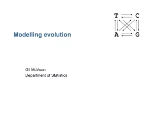
10. T C A G Modelling evolution of a single nucleotide • At a single nucleotide we only have four states (T, C, A, G). We will ignore indels. • Define the 12 rates of change from each nucleotide to every other one • We may wish to deal with changes over a fixed length of time – say one million years • The key is that we need a ‘rate’ for each possible change

11. Using the model to simulate evolution • Draw the ancestor sequence from it’s stationary distribution • Calculate the total rate at which events occur to this sequence – the sum over nucleotides, i, of the rate at which they are substituted by other nucleotides, j. • If we can treat the substitution process as a Poisson process, the time to the first substitution is exponentially distributed with rate L • The probability that a given nucleotide is chosen to be substituted by a given other nucleotide is proportional to the rate of that substitution • This allows you to choose the substitution event • Continue for as long as you want to simulate evolution for

12. An alternative approach • We have outlined a very general approach to simulating sequence evolution • For the very simple model we have discussed, we can actually make things even more efficient – which helps for inference – by taking a continuous time limit • Rewrite the transition probabilities as an instantaneous rate matrix The –S for the diagonal is such that the sum for each row is zero

13. Simulating and performing inference • The conditional distribution of the descendant nucleotide after a period of time t is given by • So the probability of observing nucleotide N1 in species 1 and N2 in species 2 is given by the appropriate element in • F is a diagonal matrix of the nucleotide frequencies in the ancestor of the two species • If F and Q are known, it is also easy to estimate t if we assume independence between sites

14. Making it simpler • Usually, various assumptions will be made to make inference easier • First, it is assumed that the matrix Q is reversible • This means that watching the process forwards in time is equivalent to watching it back in time • Consequently, summing over ancestral states is equivalent to treating one of the two sequences as ancestral • Second, it is assumed that the processes is at stationarity. This means that F is given by any column of exp(Q x t) as t → ∞ • Thirdly, further constraints are imposed on the Q matrix. • Jukes-Cantor model: all lambda’s are equal • Kimura 2-parameter model: allows different rates for transitions and transversions

15. An example • Suppose we observe the following ‘aligned’ sequence • We will use the Kimura 2-parameter model to estimate the transition-transversion ratio and the divergence time – we will assume that the rate of transversion substitution is 1.5 x 10-9 per site per year • Under the model, all sites are independent, so we can tally up the changes TGGCTGTGGACTAGTCAGCTGAGGGATATGCTAG CGATAATGCACCGGTCAGCTGAGAAATATGCAGG

16. More on inference • In calculating the likelihood we want to sum over the possible ancestral states • In effect – we have a (very simple) hidden Markov model, where the state is the ancestor and the ‘emission’ is the two daughter sequences • Because positions are independent, the likelihood is found by multiplying marginal likelihoods across sites • In effect it is a multinomial sample • We can use maximum likelihood to provide point estimates Ai Si1, Si2

17. Some estimates • For the K2P model, you actually only need to count up the number of transition and transversion differences and the total sequence length • These are sufficient statistics for the transition-transversion parameter and the divergence • There are comparable analytical expressions for estimating divergence times and model parameters for the simpler divergence models • Analytically tractability is lost as models get more complex (realistic)

18. Parameterisation using micro-evolutionary models • Most approaches to estimating divergence, etc. conflate the mutation process with the substitution process • However, it is perfectly possible to separate out the two processes • For example, estimates of the mutation process can be obtained from selectively neutral genomic regions or synonymous substitutions • This allows you to estimate the selective constraint or advantage to mutations • An area where this is applicable is in the analysis of codon usage bias, where particular codons are favoured over others for translational efficiency • McVean and Vieira (2001)

19. Making it more complex • It is easy to see how the model can be extended to more states. For example, a widely used approach to analysing coding sequences is to deal with the 64 x 64 matrix of states that are the codons (Goldman and Yang 1994) • The key point is always that parts of the sequence (nucleotides, codons) are independent • This kind of approach cannot (at least in a straightforward way) deal with context-dependent substitution rates or insertions and deletions • For example, there is a greatly elevated rate of mutation at CpG sites in vertebrates

20. Building up to trees • Analysing more sequences means thinking about the evolutionary relationships between all of them • This can (often, but not always) be represented as a tree • As before, we can utilise HMM structures to make inference efficient A1-5 Here, the HMM algorithm used to calculate the likelihood is called peeling A1-3 A1,2 A4,5 S1, S2 S4, S5 S3