Download
1 / 26
270 likes | 562 Views
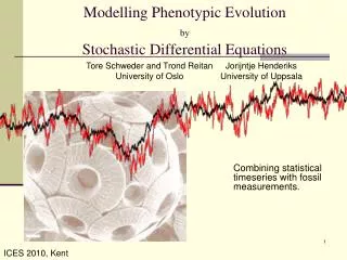
Modelling Phenotypic Evolution by Stochastic Differential Equations. Combining statistical timeseries with fossil measurements. Tore Schweder and Trond Reitan University of Oslo. Jorijntje Henderiks University of Uppsala. ICES 2010, Kent. Overview. Introduction: Motivating example:

E N D
Modelling Phenotypic Evolution byStochastic Differential Equations Combining statistical timeseries with fossil measurements. Tore Schweder and Trond Reitan University of Oslo Jorijntje Henderiks University of Uppsala ICES 2010, Kent
Overview • Introduction: • Motivating example: • Phenotypic evolution: irregular time series related by common latent processes • Coccolith data (microfossils) • 205 data points in space (6 sites) and time (60 million years) • Stochastic differential equation vector processes • Ito representation and diagonalization • Tracking processes and hidden layers • Kalman filtering • Analysis of coccolith data • Results for original model • 723 different models – Bayesian model selection and inference • Second application: Phenotypic evolution on a phylogenetic tree • Primates - preliminary results • Conclusion
Irregular time series related by latent processes: evolution of body size in CoccolithusHenderiks – Schweder - Reitan • The size of a single cell algae (Coccolithus) is measured by the diameter of its fossilized coccoliths (calcite platelets). Want to model the evolution of a lineage found at six sites. • In continuous time and ”continuously”. • By tracking a changing fitness optimum. • Fitness might be influenced by observed (temperature) and unobserved processes. • Both fitness and underlying processes might be correlated across sites. 19,899 coccolith measurements, 205 sediment samples (1< n < 400) of body size by site and time (0 to -60 my).
Our data – Coccolith size measurements 205 Sample mean log coccolith size (1 < n < 400) by time and site.
Individual samples Bi-modality rather common. Speciation? Not studied here!
Evolution of size distribution Fitness = expected number of reproducing offspring. The population tracks the fitness curve (natural selection) The fitness curve moves about, the population follow. With a known fitness, µ, the mean phenotype should be an Ornstein-Uhlenbeck process (Lande 1976). With fitness as a process, µ(t),, we can make a tracking model:
The Ornstein-Uhlenbeck process The parameters (, t, s) can be estimated from the data. In this case: 1.99, t=1/α0.80Myr, s0.12. • Attributes: • Normally distributed • Markovian • long-term level: • Standard deviation: s=/2α • α: pull • Time for the correlation to drop to 1/e: t =1/α 1.96 s t -1.96 s
One layer tracking another Red process (t2=1/2=0.2, s2=2) tracking black process (t1=1/1=2, s=1) Auto-correlation of the upper (black) process, compared to a one-layered SDE model. A slow-tracking-fast can always be re-scaled to a fast-tracking slow process. Impose identifying restriction: 1 ≥2
Process layers - illustration Observations Layer 1 – local phenotypic expression Layer 2 – local fitness optimum T External series Layer 3 – hidden climate variations or primary optimum Fixed layer
Model variants for Coccolith evolution The individual size of the algae Coccolithus has evolved over time in the world oceans. What can we say about this evolution? How fast do the populations track its fitness optimum? Are the fitness optima the same/correlated across oceans, do they vary in concert? Does fitness depend on global temperature? How fast does fitness vary over time? Are there unmeasured processes influencing fitness? Model variations: 1, 2 or 3 layers. Inclusion of external timeseries In a single layer: Local or global parameters Correlation between sites (inter-regional correlation) Deterministic response to the lower layer Random walk (no tracking)
Likelihood: Kalman filter Need a linear, normal Markov chain with independent normal observations: Process Observations The Ito solution gives, together with measurement variances, what is needed to calculate the likelihood using the Kalman filter: and
Kalman smoothing (state estimation)ML fit of a tracking model with 3 layers North Atlantic Red curve: expectancy Black curve: realization Green curve: uncertainty Snapshot:
Inference • Exact Gaussian likelihood, multi-modal • Maximum likelihood by hill climbing from 50 starting points • BIC for model comparison. • Bayesian: • Wide but informative prior distributions respecting identifying restrictions • MCMC (with parallel tempering) + Importance sampling (for model likelihood) • Bayes factor for model comparison and posterior probabilities • Posterior weight of a property C from posterior model probabilities
Model inference concerns Concerns: • Identification restriction: increasing tracking speed up the layers • In total: 723 models when equivalent models are pruned out) Enough data for model selection? • Data Simulated from the ML fit of the original model • Model selection over original model plus 25 likely suspects. • correct number of layers generally found with the Bayesian approach. • BIC seems too stingy on the number of layers.
Results, original model 3 layers, no regionality, no correlation
Summary • Best 5 models in good agreement. (together, 19.7% of summed integrated likelihood): • Three layers. • Common expectancy in bottom layer . • No impact of exogenous temperature series. • Lowest layer: Inter-regional correlations, 0.5. Site-specific pull. • Middle layer: Intermediate tracking. • Upper layer: Very fast tracking. Middle layers: fitness optima Top layer: population mean log size
Phenotypic evolution on a phylogenetic tree: Body size of primates
Why linear SDE processes? • Parsimonious: Simplest way of having a stochastic continuous time process that can track something else. • Tractable: The likelihood, L() f(Data | ), can be analytically calculated by the Kalman filter or directly by the parameterized multi-normal model for the observations. ( = model parameter set) • Some justification from biology, see Lande (1976), Estes and Arnold (2007), Hansen (1997), Hansen et. al (2008). • Great flexibility, widely applicable...
Further comments • Many processes evolve in continuous rather than discrete time. Thinking and modelling might then be more natural in continuous time. • Tracking SDE processes with latent layers allow rather general correlation structure within and between time series. Inference is possible. • Continuous time models allow related processes to be observed at variable frequencies (high-frequency data analyzed along with low frequency data). • Endogeneity, regression structure, co-integration, non- stationarity, causal structure, seasonality …. are possible in SDE processes. • Extensions to non-linear SDE models… • SDE processes might be driven by non-Gaussian instantaneous stochasticity (jump processes).
Bibliography • Commenges D and Gégout-Petit A (2009), A general dynamical statistical model with causal interpretation. J.R. Statist. Soc. B, 71, 719-736 • Lande R (1976), Natural Selection and Random Genetic Drift in Phenotypic Evolution, Evolution 30, 314-334 • Hansen TF (1997), Stabilizing Selection and the Comparative Analysis of Adaptation, Evolution, 51-5, 1341-1351 • Estes S, Arnold SJ (2007), Resolving the Paradox of Stasis: Models with Stabilizing Selection Explain Evolutionary Divergence on All Timescales, The American Naturalist, 169-2, 227-244 • Hansen TF, Pienaar J, Orzack SH (2008), A Comparative Method for Studying Adaptation to a Randomly Evolving Environment, Evolution 62-8, 1965-1977 • Schuss Z (1980). Theory and Applications of Stochastic Differential Equations. John Wiley and Sons, Inc., New York. • Schweder T (1970). Decomposable Markov Processes. J. Applied Prob. 7, 400–410 Source codes, examples files and supplementary information can be found at http://folk.uio.no/trondr/layered/.