Modelling Diffuse Subcellular Protein Structures as Dynamic Social Networks
350 likes | 366 Views
This Master's thesis explores the use of network models to study the behavior of diffuse organellar structures within cells. The thesis focuses on solid structures such as cells, nuclei, and microorganisms, and applies graph theory and social network analysis to understand their behavior.

Modelling Diffuse Subcellular Protein Structures as Dynamic Social Networks
E N D
Presentation Transcript
MODELLING DIFFUSE SUBCELLULAR PROTEIN STRUCTURES AS DYNAMIC SOCIAL NETWORKS Master’s Thesis By Andrew Durden Under the Direction of: Shannon Quinn Frederick Quinn Tianming Liu
Ornet (Organellar Network) • Fit network models to diffuse organellar structures to study cell behavior
Advancements in Medical Imaging and Modeling • Automated microscopes increase quantity of data • Manual annotation had been the norm • Efforts in automated image analysis exploded • BioImageXD • Icy • Fiji • Deep Learning has become the cutting edge (U-net)
Focus on Solid Bodies • Objects like full cell, nuclei, microorganisms all exhibit solid structure • These solid forms are more commonly used for teaching and for algorithmic research Image sources: Top: (Ljosa & Carpenter 2009) Bottom: ISBI cell tracking competition (Maska et al. 2014) (Ulman et al. 2017)
Significance • Improve our ability to describe dynamic cell morphology • Further understand effects of various stimuli on mitochondrial behavior • Mitochondrial misbehavior have been shown to be: • Causative in neurogenerative diseases • Evidence of bacterial infections Image source: (Stavru et al. 2011)
Our Dataset • HeLa cells transfected with DsRed2-Mito-7 • Images were captured every ten seconds for the length of the video. • Three morphologies • Fragmented (LLO) • Control/Wild Type • Hyperfusion (Mdivi1)
Social Networks • Started in sociology • Became more popularized: • 6 degrees of separation • Kevin Bacon Number • Have been applied to various fields: • Ecology • Internet Topology • Microbiology Image source: (Milgram 1967)
Graph Theory • Set of Nodes • Connected by edges • Directed or Undirected • Weighted or Unweighted • Differing structures • Random Network • Scale Free Networks • community structures • Graph Theory Based Metrics • Clustering Coefficient • Network Diameter
Proposed Pipeline • Segmentation • Extract • Fit Nodes • Determine Affinities/Edges • Network Analysis
Thresholding • The traditional approach • Has two main variants • Global: single value • Adaptive: multivalue • used for binarization of greyscale images Image source: (Ljosa & Carpenter 2009)
Adaptive Thresholds • Fit multiple thresholds to regions of the image • Allows for better results when lighting or background varies • Examples: • Neighborhood approach • Surface Fitting Image source: (Chan et al. 1998)
Global Thresholding • Uses a single threshold • Works best in uniform images • Variety of methods: • Histogram shape • Pixel value clustering • Manually set values Image source: (Chan et al. 1998)
ISODATA results • Process: • Applied global threshold • Dilated and removed small holes • Applied convex hull to each component • Shortcomings: • Separates single cell into multiple mask • Merges adjacent cells into single mask
Deformable Contours • Requires initial contours • Manually drawn seeds • Snakes Model • Localize edges using energy-minimization • Iteratively adjusts localization until it reaches energy equilibrium • Can be used to track low motility objects Image source: (Kass et al. 1988)
Our Segmentation • Merges thresholding and deformable contours • Uses previous frame as seed • Determines a tight contour within the seed using global threshold • Dilates that tight contour iteratively • Eliminates overlaps during dilation
Creating Nodes • Initially used connected component analysis • Pros • Grouped protein together based on vicinity • Low processing time • Cons • Data is lost in thresholding • Relationship between nodes is difficult to discern
Gaussian Mixture Model • Fits a mixture of gaussians to model data • Follows and expectation-maximization algorithm • Computes each data points probability of belonging to each gaussian • Adjust Gaussian parameters to maximize probabilities • Repeat until convergence
Preprocessing for GMM • First we removed noise with a Gaussian Smoothing Filter • Next we need to view the image as a probability density function • Normalize the intensities to sum to one • Determine initial mixture parameters • Max filter to determine initial means and number of components • Covariance uses the covariance of the pixel neighborhood
Creating Nodes • Modeled protein with a Gaussian Mixture Model • Pros: • Incorporates all of the data • Gives spatial covariance of the communities • Can use previous frame to initialize • Cons: • Higher processing time • Preprocessing steps require hyperparameters
Creating Edges • Initially used a radial-basis function with a manual threshold • Uses the Euclidean distance between two nodes • Didn’t take covariance into account when determining Neighborhood • Altered this method by using the covariance the direction of the connection to replace the manual threshold • More data-driven • Still induces sparsity • Accounts for directionality of components • Cons • Was overly dependent on distance • Point wise comparison
Creating Edges • Moved towards a probability based metric • The weight of the connection between A and B is the probability of the mean of B in the distribution A. • Accounts for directionality in creating the weights • Created an Asymmetric graph • Only offered pointwise comparison
Creating Edges • Applies divergence metrics as affinity • Kullback-Leibler (KL) divergence • Jensen-Shannon (JS) divergence • Takes full gaussian distribution into account • Allows for both asymmetric and symmetric affinities
Affinity Distribution • Distribution of affinities over time between Wild type (top) and LLO (bottom) • Using probability based affinities • Negative log of the affinity
Spectral Decomposition • Apply a heat kernel to convert JS divergence to similarities • Create a graph Laplacian from similarity matrix • Use Spectral Decomposition to factor the Laplacian • Viewed Eigenvalues over time
Model Limitations and Next Steps • Next steps in analysis • Laplacian Gradients • Clustering Eigenvalue changes • Look into Connectivity, cliques, and other classic graph metrics • Model limitations and future improvements • Incorporate a uniform component to account for background noise • Combat node collapse in LLO data • Incorporate dynamic node quantity • Fully automated segmentation
Conclusion • We have presented a pipeline for producing quantitative models of diffuse subcellular protein structure • We have shown how this model can evolve overtime to account for changing morphologies • We have shown how the properties of the network can be interpreted to provide biological insights
Acknowledgements • Acknowledgements • This project was supported in part by a grant from the National Science Foundation (#1458766) • I would like to thank MojtabaFazli and Shannon Quinn for their help and guidance on this project • I would also like to thank Allyson Loy, Barbara Reaves, Abigail Courtney, Chakra Chennubhotla, Fred Quinn, Brittany Dorsey, and Chinasa Okolo. Their work with the Ornet project has made my research possible
References Ljosa V, & Carpenter A E (2009). Introduction to the quantitative analysis of twodimensional fluorescence microscopy images for cell-based screening. PLoS computational biology, 5(12), e1000603. Maška M, Ulman V, […], Ortiz-de-Solorzano C. (2014) A benchmark for comparison of cell tracking algorithms, Bioinformatics, Volume 30, Issue 11, 1 June 2014, Pages 1609–1617, https://doi.org/10.1093/bioinformatics/btu080 Ulman V, Maška M, […] Ortiz-de-Solorzano C. (2017) An objective comparison of cell-tracking algorithms. Nature Methods 14, 1141-1152 Chan F H Y, Lam F K, Zhu H. (1998). Adaptive Thresholding by Variational Method. IEEE Transactions on Image Processing, v. 7 n. 3, p. 468- 473 Kass M, Witkin A, Terzopoulos D. (1988) Snakes: Active Contour Models. International Journal of Computer Vision, 1 (4): 321. doi:10.1007/BF00133570. Milgram S (1967). The Small-World Problem. Psychology Today vol 1, no 1, 61-67