Download
1 / 37
370 likes | 527 Views
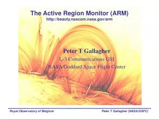
The Active Region Monitor (ARM) http://beauty.nascom.nasa.gov/arm. Peter T Gallagher L-3 Communications GSI NASA Goddard Space Flight Center. What ARM does and does not do. Extremely simple approach based on mature technologies IDL, Perl, C-shell, HTML No advanced image processing … yet

E N D
The Active Region Monitor (ARM)http://beauty.nascom.nasa.gov/arm Peter T Gallagher L-3 Communications GSI NASA Goddard Space Flight Center Peter T Gallagher (NASA/GSFC)
What ARM does and does not do • Extremely simple approach based on mature technologies • IDL, Perl, C-shell, HTML • No advanced image processing … yet • No distributed computing Peter T Gallagher (NASA/GSFC)
Basic Architecture of the Active Region Monitor (ARM) Apache Web Server http://beauty.nascom.nasa.gov/arm Data Processing And Archiving C-shell IDL Perl IDL sockets SOHO EIT/MDI GONG+ Mags BBSO H-alpha NOAA SRS NOAA SXI SOLIS FASR Peter T Gallagher (NASA/GSFC)
Physical Motivation - The Magnetic Field • Line of sight B-field • Zeeman effect • ±2000 G • Corona: < 1 • Photosphere: > 1 Peter T Gallagher (NASA/GSFC)
B The Induction Equation • The evolution of magnetic fields in solar active regions can be described by the magnetic induction equation • Rm is 108 to 1010 in photosphere. • Field “frozen” into the plasma. • Field is advected by bulk plasma motions Plasma Peter T Gallagher (NASA/GSFC)
ARM Extensions Include measures that are sensitive to the small-scale nature of energy storage and release in the solar atmosphere. • Fractal dimension: relates to the active region complexity. • Field gradient: indicative of pressure build-up in the photosphere. • Neutral lines: related to energy release locations. • Emerging flux regions: can act as energy release triggers. • Wavelet analysis: diagnostic of small and large scale morphology. Peter T Gallagher (NASA/GSFC)
Fractal Dimension - Motivation • Turbulent plasma motions => Fields follow a random walk. • Lawrence and co-workers find that line-of-sight fields scale in a self-similar and fractal manner. • Correlation between Mt. Wilson classification and the fractal dimension (Gallagher, McAteer, & Ireland, 2003). • Tao et al. (1995) showed that the advection of magnetic flux tubes by random motions results in a spatial distribution of flux which is fractal. • Percolation theory: geometry of flux concentrations on the solar surface naturally results in fractal dimensions consistent with observational values (Vlahos et al., 2002; Schrijver et al., 1992; Seiden & Wentzel, 1996). • Measuring the fractal dimension of an active region magnetic field is an essentially global investigation of the scaling properties of the magnetic field. Peter T Gallagher (NASA/GSFC)
Fractal Dimension - Methods • Box-Counting Dimension (Mandelbrot): • The box-counting dimension can then be then determined from the slope, • Perimeter-Area Dimension (Hausdorff): • The perimeter-area dimension can then be obtained from, Peter T Gallagher (NASA/GSFC)
Fractal Dimension - Example • ~ 1.0 - 1.2 • ~ 1.2 - 1.4 • ~ 1.4 - 1.6 • ~ 1.5 - 1.7 • Error ~ ± 0.1 Peter T Gallagher (NASA/GSFC)
Horizontal Gradient - Motivation • It is because the field is frozen into the plasma in the photosphere that large transverse gradients are observed across the neutral line of large spots (Patty & Hagyard, 1986; Zhang et al., 1994). • Converging photospheric flows sweep opposite polarity fields towards the neutral line of the . • Over a period of hours, the continued concentration of opposite polarities in a relatively small area leads to strong transverse gradients (Gallagher, Moon, & Wang 2002). • energy_buldup (hrs - days) >> energy_resease (secs - mins) • An instability in the corona results in the release of stored (Lin & Forbes, 2001; Priest & Forbes, 1990) Peter T Gallagher (NASA/GSFC)
Horizontal Gradient - Method • The horizontal gradient of the line-of-sight field, Bz(x,y) can be calculated using, • The magnitude of the gradient can then be evaluated using, • While the direction can be found from, Peter T Gallagher (NASA/GSFC)
Horizontal Gradient - Example • Gradients are large for large fields in close proximity. Peter T Gallagher (NASA/GSFC)
Neutral Line - Motivation • Energy can be stored in the corona when sunspots of opposite polarity are pushed together, thereby forming an extended current sheet above the neutral line in the overlying magnetic field (Parker, 1963; Roumeliotis & Moore, 1993). • “Break-out” model: gradual shearing motion both across and along the neutral line, can result in the formation of unstable arcades structures in the solar corona, which can then erupt (Antiochos, Devore, & Klimchuk, 1999). • Observational flare signatures in neutral line morphology (Zharkova et al., this meeting). Peter T Gallagher (NASA/GSFC)
Neutral Line - Method • The magnetogram is first smoothed using a boxcar filter - this removes much of the statistical noise which would otherwise limit the effectiveness of subsequent steps. • Contours of constant magnetic flux are then overlayed on the magnetogram at the zero Gauss level. • Pixels along these contours are then extracted and used to create a binary image, with pixels along the neutral line have a value of 1, and all others being set to 0. • This binary mask can then be used to extract gradient values along the neutral line by multiplying it with the gradient map. Peter T Gallagher (NASA/GSFC)
Neutral Line - Example Peter T Gallagher (NASA/GSFC)
Emerging/Submerging Flux Regions (ESFRs) - Motivation • Filament eruptions can be triggered by ESFRs (Feynman & Martin, 1995). • Major flares tend to be associated with new flux emergence (Tang & Wang, 1993; Wang et al. 2003; Zharkova). • CMEs, which may be associated with filament eruptions and/or flares, may also be triggered by ESFRs (Green et al., 2003). • Emerging flux model (Heyvaerts, Priest, & Rust, 1977). • Flux-rope destabilization by flux injection (Krall, Chen, & Santoro, 2000). Peter T Gallagher (NASA/GSFC)
Emerging/Submerging Flux Regions (ESFRs) - Method • Automatic monitoring of ESFRs is therefore extremely important to tracking and predicting solar activity. • ESFRs will be monitored using full-disk MDI and GONG magnetograms in conjunction with a near real-time running-difference algorithm. • Each newly processed magnetogram can be differentially rotated to the location of the previously processed magnetogram and subtracted. • ESFRs are then identified as areas in the difference image showing large deviations (say, 3 ) above the mean difference level. • ESFR frequency and location will then be cataloged and overplotted on images obtained at EUV or X-ray wavelengths, for example. Peter T Gallagher (NASA/GSFC)
Emerging Flux Regions (ESFRs) - Example Peter T Gallagher (NASA/GSFC)
Emerging Flux Regions (ESFRs) - Example Peter T Gallagher (NASA/GSFC)
Wavelets - Motivation • Measuring the fractal dimension of an active region magnetic field is an essentially global investigation of the scaling properties of the magnetic field. • Such an approach could easily overlook spatially localized scale features, such as the emergence/submergence of flux tubes. Such locations are of especial interest in flare physics and are also vital in detailing the evolutionary path of active region development. • A wavelet analysis of magnetograms can discriminate such regions. • It is this lengthscale content which is crucial for theories of active region development. Peter T Gallagher (NASA/GSFC)
Wavelets - Method • Test the suitability of various wavelet decomposition schemes (Haar, à trous, etc.) • Find and characterize the local scale content of magnetograms and analyze this in the context of flare occurrence locations, times, rates and flux emergence/submergence. • Characterize the evolution of spatial distribution of magnetogram scale content via entropy measures. Peter T Gallagher (NASA/GSFC)
Wavelets - Example Peter T Gallagher (NASA/GSFC)
Summary of Modifications Peter T Gallagher (NASA/GSFC)
Potential Field Extrapolations - Motivation • Energy release occurs in the corona. • Coronal field topology is crucial to understanding and predicting activity (Antiochas, 1990; Aulanier et al. 2000). • Fast and easy to implement - IDL code to be added to SSW. Peter T Gallagher (NASA/GSFC)
Potential Field Extrapolations - Method • In equilibrium, and in the absence of flows, the magnetohydrostatic force balance equation can be written, where P is the gas pressure, and FG is the force due to gravity. If the pressure gradients and gravity are negligible, we have so that the current must be parallel to the magnetic field. In other words, where is a function of position within the force-free magnetic field. The simplest solution to this equation can be obtained when = 0. This extrapolated field is then current-free, or potential. Peter T Gallagher (NASA/GSFC)
Potential Field Extrapolations - Example - simple bipolar topology - complex multipolar topology Peter T Gallagher (NASA/GSFC)
Conclusions • Improve stability and reliability of ARM. • Include advance image processing techniques. • Incorporate a potential field extrapolation and visualization tool into ARM. • FITS data products. • ARM and VSO/EGSO? Peter T Gallagher (NASA/GSFC)