Download
1 / 18
180 likes | 207 Views
This article explains the concept of z-scores and their representation in a distribution, as well as how they are used in hypothesis testing. It also discusses the significance level and the interpretation of significant results. Additionally, it covers different types of t-tests and their applications, along with making inferences about the population using sampling distributions and the Central Limit Theorem.

E N D
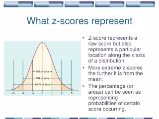
What z-scores represent • Z-score represents a raw score but also represents a particular location along the x axis of a distribution. • More extreme z-scores the further it is from the mean. • The percentage (or areas) can be seen as representing probabilities of certain score occurring.
Hypothesis testing and z scores • Research hypothesis presents a statement of the expected event. e.g. 12th graders and 9th graders will differ on the ABC memory test. • We use statistical tools to evaluate how likely that event is. • So if we find a z score that is extreme, we like to say that the reason for the extreme score is something to do with treatments (ABC memory test) and not just chance.
How extreme is “extreme”? • Less than 5 % chance of occurring (p <.05) • Less than 1% chance of occurring (p<.01) • Less than .1% chance of occurring (p<.001)
Significance level p<.05 “there was a significant differences in the memory test result between 12th graders and 9th graders Meaning: • The probability of getting the difference between 12th graders and 9th graders in the sample BY CHANCE was less than 5%. • Therefore, can concluded that the differences is due to some systematic influence (grade difference) and not due to chance.
The Concept of Significance “There is a significant difference in attitude toward ‘on-line dating service’ between students and non-students (p. <.05) ” • What does it mean by “significant” • It means that any difference between the attitudes of the two groups is due to some systematic influence and not due to chance.
t(ea) for Two: Test between the Means of Different Groups • When you want to know if there is a ‘difference’ between the two groups in the mean • Use “t-test”. • Why can’t we just use the “difference” in score? • Because we have to take the ‘variability’ into account. • t = difference between group means sampling variability
One-Sample T Test • Evaluates whether the mean on a test variable is significantly different from a constant (test value). • Test value typically represents a neutral point. (e.g. midpoint on the test variable, the average value of the test variable based on past research)
Independent-Sample T test • Evaluates the difference between the means of two independent groups. • Also called “Between Groups T test” • Ho: 1= 2 H1: 1= 2
Independent Samples Test Levene's Test for Equality of Variances t-test for Equality of Means 95% Confidence Interval of the Difference Mean Std. Error F Sig. t df Sig. (2-tailed) Difference Difference Lower Upper Current Salary Equal variances 119.669 .000 -10.945 472 .000 -15409.86 1407.906 -18176.4 -12643.3 assumed Equal variances -11.688 344.262 .000 -15409.86 1318.400 -18003.0 -12816.7 not assumed
APA write-up of Independent Sample t-test The independent-sample t-test was conducted to evaluate the hypothesis that there is a significant difference in the salary between male and female. The test was significant, t(344.262)= -11.688, p<.001.
Paired-Sample T test • Evaluates whether the mean of the difference between the paired variables is significantly different than zero. • Applicable to 1) repeated measures and 2) matched subjects. • Also called “Within Subject T test” “Repeated Measures T test”. • Ho: d= 0 H1: d= 0
APA write-up of Paired-sample t-test • A paired sample t-test was conducted to evaluate whether there is a significant change in the level of anxiety between trail 1 and trail 2. The result indicated that the mean anxiety level at trial 1 was significantly higher (M=16.50, SD=2.07) then the mean anxiety level at trial 2 (M=11.50, SD=2.43), t(11)=7.54, p<.001.
Making Inference About the Population • Sampling Distribution • A frequency distribution of a sample statistics. • 1) Select repeated, independent samples, 2) compute a value of the statistic for each sample, 3) identify the frequency distribution of the sample statistics. • Standard Error • Standard deviation of the Sampling Distribution
Making Inference About the Population • The Central Limit Theorem • As long as you have a reasonably large sample size, the sampling distribution of the mean will be normally distributed. • Average of the sample statistics = Average of population value. • When we conduct a significance test, we are checking if the sample statistic is an anomaly or not.
Type I Error • Type I error happens when the null hypothesis is rejected even though it is true. • Level of significance: The risk of making a Type I error. • alpha level, p level. • p < .05 : • The risk of making a Type I error was set at .05 (5%), and the null hypothesis was rejected in favor of the alternative hypothesis. • The probability of rejecting the null hypothesis by chance and making a Type I error is lower than .05.
Type II Error • Type II error: If the alternative hypothesis is true, but the decision maker decides to stick with the null hypothesis. • Risk of making Type II error = Beta (β)