Download
1 / 21
210 likes | 289 Views
Explore how recurrence analysis enhances traditional fisheries science by uncovering non-linear dynamics and interdependencies within marine ecosystems. Discover methods like change point detection and Takens' theorem for insightful time series analysis.

E N D
Recurrence analysis and Fisheries Fisheries as a complex systems Traditional science operates on the assumption that natural systems like fish populations exist in balance. But in reality they are in constant flux - spiking up and down, with many overlapping cycles - and can be upset by even tiny changes. Now there are a growing emphasis both on interdependencies in large marine ecosystems and on the non-linear or chaotic changes that are prominent features of these systems.
Recurrence analysis and Fisheries Time series analysis The main aims when investigate a nonstionarity time series are • Characterisation. When a dynamics underlying a non stationarity of time series is similar at beginning and end but not at middle, the aim of techniques which analyse the non stationarity is to select this information in convenient form. • Prediction. An accurate predictions (Priestley 1988, Stark 1993,Weigend et alt. 1995) for a non stationariety time series can be obtained modifying prediction algorithms. This procedures is strongly connected to characterisation and modelling time series.
Recurrence analysis and Fisheries Time series analysis • Change point detection. The dynamics which characterises a time series can have a single point of change. The objective of time series analysis is to identify this change point (Lima 1995, Kennel 1996). • Hypothesis testing. In some case there may be reason to believe that a time series is stationary. The objective is to develop hypothesis tests for the null hypothesis. If the null hypothesis is accepted one can then have confidence in applying techniques of stationarity time series analysis. The recurrence plots provide an unified framework for addressing all those objectives
Recurrence analysis and Fisheries Recurrence plots approach The recurrence plots are a visualisation tool for analysing experimental data. The basic feature of this tool is to reveal correlation in the data that are not easily detected in the original time series. It not requires any assumptions on the stationarity of time series, then Rps are particularly used in the analysis of systems whose dynamics may be changing. Some author (Zbilut, Webber, giuliani, Trulla) have highlighted that RPs can be compared to classical approaches for analysing chaotic data, especially in its ability to detect bifurcation. The fundamental assumption underlying the idea of the recurrence plots is that an observable time series (a sequence of observations) is the realization of some dynamical process, the interaction of the relevant variables over time
Recurrence analysis and Fisheries Takens theorem This theorem says that it can recreate a topologically equivalent picture of the original multidimensional system behavior by using the time series of a single observable variable. The basic idea is that the effect of all the other (unobserved) variables is already reflected in the series of the observed output. Furthermore, the rules that govern the behavior of the original system can be recovered from its output.
Recurrence analysis and Fisheries Recurrence plots approach The recurrence plots basis on the reconstruction space state. The reconstruction space state is the first steps to analyse a time series in a context of dynamical systems theory when the only information is contained in a time series. This approach is founded on flow of information from unobserved variables to observed variables “past and future of a time series contain information about unobserved state variables that can be used to define a state at the present time” (M. Casdagli, S. Eubank. J. D. Farmer, J. Gibson, 1991). Although the theoretical approach of Takens’ theorem highlight that the choice of coordinate which representing an embedding is indifferent, in practical analysis it is demonstrated as the choice of coordinate affects the predictions result.
Recurrence analysis and Fisheries Methods for reconstruction space state The methods for reconstruction space state are: • Delay coordinates • Derivative coordinates • Global principal value decomposition Although all three methods are applied for the reconstruction space state, the delay coordinates is most used (VRA basis on this method).
Recurrence analysis and Fisheries Delayed coordinate In VRA, a one-dimensional time series from a data file is expanded into a higher-dimensional space, in which the dynamic of the underlying generator takes place. The delayed coordinate embedding recreates a phase space portrait of the dynamical system under study from a single (scalar) time series. To expand a one-dimensional signal into an M-dimensional phase space, one substitutes each observation in the original signal X(t) with vector y(i) = {x(i), x(i - d), x(i - 2d), … , x(i - (m-1)d}, i is the time index, m is the embedding dimension d is the time delay. As a result, we have a series of vectors: Y = {y(1), y(2), y(3), …, y(N-(m-1)d)}, N is the length of the original series. The idea of such reconstruction is to capture the original system states at each time we have an observation of that system output. Each unknown state S(t) at time t is approximated by a vector of delayed coordinates Y(t) = { x(t), x(t - d), x(t - 2d), … , x(t - (m-1)d }
Recurrence analysis and Fisheries Spatio-Temporal Entropy Spatio-Temporal Entropy (STE) measures the image "structureness" in both space and time domains. Essentially, it compares the global distribution of colors over the entire recurrence plot with the distribution of colors over each diagonal line of the recurrence plot. The higher the combined differences between the global distribution and the distributions over the individual diagonal lines, the more structured the image is. In physical terms, this quantity compares the distribution of distances between all pairs of vectors in the reconstructed state space with that of distances between different orbits evolving in time. The result is normalized and presented as a percentage of "maximum" entropy (randomness). That is, 100% entropy means the absence of any structure whatsoever (uniform distribution of colors, pure randomness), while 0% entropy implies "perfect" structure (distinct color patterns, perfect "structureness" and predictability). Thus, the following range of spatio-temporal entropy should be expected for different signals. Notice that the closer are the values of the embedding dimension and the time delay to the “true”values, the lower is the entropy of the recurrence plot
Recurrence analysis and Fisheries Embedding dimension The analytical methods for estimating the embedding dimension is the false nearest neighbours method. The False Nearest Neighbors is a method of choosing the minimum embedding dimension of a one-dimensional time series, suggested by Kennel et al. This method finds the nearest neighbor of every point in a given dimension, then checks to see if these points are still close neighbors in one higher dimension. The percentage of False Nearest Neighbors should drop to zero when the appropriate embedding dimension has been reached.
Recurrence analysis and Fisheries The False Nearest Neighbors
Recurrence analysis and Fisheries The False Nearest Neighbors Ideally, d should be large enough to unfold the system trajectories from self-overlaps, but not too large, the noise will amplify. The rule of thumb is to set m to m<= 2N+1, where N is the number of operating variables, or degrees of freedom, in the dynamical system under study
Recurrence analysis and Fisheries Delay time The analytical methods for estimating the delay time is the mutual information function. Mutual information is a general measure, based on information theory, of the extent to which the values in a time series can be predicted by earlier values. It is not limited to linear dependence as is the autocorrelation function. It measures the state predictability or the memory of a system.
Recurrence analysis and Fisheries Mutual information function Mutual information function can be used to determine the “optimal” value of the time delay for the state space reconstruction. The idea is that a good choice for the time delay T is one that, given the state of the system X(t), provides maximum new information with measurement at X(t+T). Mutual information is the answer to the question, "Given a measurement of X(t), how many bits on the average can be predicted about X(t+T)?" A graph of I(T) starts off very high (given a measurement X(t), we know as many bits as possible about X(t+0)=X(t)). As T is increased, I(T) decreases, then usually rises again. It is suggested that the value of time delay where I(T) reaches its first minimum be used for the state space reconstruction.
Recurrence analysis and Fisheries Mutual information function an example The mutual information I(k) (Farmer1982 ) is a generalization of the correlation function. It measures the state predictability or the memory of a system, represented by a sequence of certain symbols. In the following we consider sequences in which only two different symbols (say 0 and 1) can occur. Then, I(k) defined by quantifies the average dependence of two symbols over k time steps, where piis the probability of the symbol of a symbol string, and is the joint probability that the symbol and steps k later the symbol occurs. In particular, peaks in I(k) exhibit the levels of memory quantitatively. This description is especially appropriate for nonlinear systems because the joint probabilities reflect more general dependencies within a symbolic string than the autocorrelation function.
Recurrence analysis and Fisheries Mutual information function an example (continued) In the case of white noise, mutual information I(k) vanishes for all ,reflecting that white noise is a process without any memory. Periodic processes are characterized by peaks at the multiples of the period in k . Chaotic regimes yield a decrease of mutual information I(k) with growing k (Hempelmann and Kurths 1990). Note that structures of particular interest here are detected by mutual information but not by autocorrelation function. For short sequences, artifacts may occur in the calculation of I(k). Therefore, we propose a method to judge the statistical significance of peaks in I(k) by a statistical, semi-empiric method, called randomization (e.g. Random 1990).
Recurrence analysis and Fisheries Application fisheries data Delay 1 Dimension 1
Recurrence analysis and Fisheries Application fisheries data Delay 4 Dimension 2
Recurrence analysis and Fisheries Application fisheries data Spatio-Temporal Entropy Delay 4 Dimension 2
Recurrence analysis and Fisheries Application fisheries data Delay 10 Dimension 6
Recurrence analysis and Fisheries Application fisheries data Spatio-Temporal Entropy Delay 10 Dimension 6