Operations on Complementary Edge Binary Decision Diagrams
Learn how to perform key operations in Canonical Complementary Edge Binary Decision Diagrams and convert from ROBDD form. Includes complementation, reordering, tautology, and more.


Operations on Complementary Edge Binary Decision Diagrams
E N D
Presentation Transcript
Operations on Complementary Edge Binary Decision Diagrams EE 552 Instructor: Dr. James Ellison Kenny Liu KennyLiu@usc.edu July 22nd, 2003
Introduction From the text, we are familiar with performing various operations in the ROBDD (Reduced Order Binary Decision Diagram) form. There were various notations mentioned in the text and we will be focusing on the CCE BDD (Canonical Complementary Edge Binary Decision Diagram) form. The presentation will show and prove methods of performing the operations we are already familiar with in the ROBDD form, but now in the CCE BDD form.
Introduction • The operations mentioned will include: • complementation • finding the product of sums (POS) and sum of products (SOP) representation • reordering variables • dual • cofactor representation • tautology and satisfiability • disjunctive composition
Conversion from ROBDD to CCEBDD f = xz’+x’yz’ f x x Here we have our basic ROBDD form. We will be converting to CCE BDD form through a series of steps. y y z z • Change all dotted lines (0-edges) into a line with a clear circle. 0 1 0 1 After Step 1 ROBDD
Conversion from ROBDD to CCEBDD f f x x • All lines going to the 1-leaf are represented with leaf-less notation • All lines going to the 0-leaf are represented as leaf-less and with a solid dot on that branch. y y z z 0 After Step 3 After Step 2
Conversion from ROBDD to CCEBDD f f 4) The next step is to remove all solid dots that are on lines without clear dots, in our example we have just one such case. We are only allowed to remove this solid dot if we add solid dots to all other branches of the node. x x y y z z After Step 3 After Step 4
Conversion from ROBDD to CCEBDD f f x x Repeat Step 4 y y z z After Step 4 After Step 4
Conversion from ROBDD to CCEBDD f f 5) In this step, any edge with 2 solid dots can cancel out. The text also takes another step in which to represent an edge with a solid dot and clear dot as just a solid dot since we know it can only appear on zero edges anyways, but we will skip this step to make it easier to understand as we perform operations later. x x y y z z After Step 4 After Step 5
Conversion from ROBDD to CCEBDD f Here we have our final CCEBDD. We can see a major difference from an ROBDD in that it has a root edge which is the branch above the root node. Through this method of notation, the solid dots complement the portion of the function from the child node down. We will go into more detail of how this works later. x y z After Step 5
Summary of CCEBDD • Basic Properties of CCEBDD form: • Has a root edge which may have a solid dot. • 0-edges are represented as lines with clear dot. • There are only 1 leaves, 0-leaves are replaces with 1-leaves with a solid dot. • No solid dots may appear on positive edge. Cancel out with method shown previously. • Two solid dots on the same branch cancels each other out. • There is one unique CCEBDD for a boolean function for a particular ordering of its variables.
Basic Operation on CCEBDD f The main operation we must be familiar with before we proceed is how to obtain the boolean function from a given CCEBDD. For Sum of Products in ROBDD, we are used to taking each possible path down to the 1-leaf, but here the process will be a little different. Instead, the path we are looking for must contain an even number of solid dots (ex. 0,2,4,6 etc.). If there is a solid dot on the root edge, we must take that into account for each path. We can verify our results with our original ROBDD. x y z
Basic Operation on CCEBDD f In our simple example there is only two such paths which is highlighted in red and pink. Each path contains 2 dots and each path represents part of the function. Sum of Products (even number of dots): (red highlight, 2-dots, path = x, z’) = xz’ (pink highlight, 2-dots, path = x’, y, z’) = x’yz’ Therefore f = xz’ + x’yz’ x y z
Complementation f = x+x’y+x’y’z’ f’ = x’y’z Complementation in ROBDD form is simple because all that needs to be done is to switch the 1-leaf with the 0-leaf. Actually complementation in CCEBDD form is just as easy but we will show the process with an example. Here we have a function in ROBDD and its complement. x x y y z z 0 1 1 0
Complementation We will now convert the ROBDD into a CCEBDD both regular and complemented functions to compare. f = x+x’y+x’y’z’ f f x x x y y y z z z 0 1
Complementation f’ = x’y’z f’ = x’y’z f’ = x’y’z x x x y y y z z z 1 0
Complementation By visually comparing the two CCEBDD’s, we can see that the complemented version just has the added solid dot on the root edge. With the solid dot representing the complementation of everything below it, it makes sense that a solid dot above the root node will complement the entire function. f = x+x’y+x’y’z’ f’ = x’y’z x x y y z z
Product of Sums We are already familiar with finding the Sum of Products function of a given CCEBDD in which we take each path that contains an even number of solid dots as a group of products with each group summed together. To find the Product of Sums function, it’s basically the same process, just with the 0-leaf, and so in CCEBDD form we look for paths with odd number of solid dots. We also need to complement each node as we did when finding Product of Sums for ROBDD’s.
Product of Sums Going back to our original example, we have 3 paths with an odd number of solid dots. Product of Sums (odd number of dots): (red highlight, 1-dot, path = x, z) = x’+z’ (pink highlight, 1-dot, path = x’, y, z) = x+y’+z’ (yellow highlight, 1-dot, path = x’, y’) = x+y Therefore f = (x’+z’)(x+y’+z’)(x+y) f x y z
Reordering of Variables The process in which we reorder variables in CCEBDD is very much the same as when we reorder variables in ROBDD. The leaves and nodes which involve the 2 variables to be reordered must be fully expanded keeping in mind that the 0-edge is always on the left. Afterwards, the variables can be switched along with the 2 leaf values in the expanded tree. a b After swap a a b b N1 N3 N2 N4 N1 N2 N3 N4
Reordering of Variables In the following example, we will swap the y and z variable. f f x x We first expand the CCEBDD y y y z z z z z
Reordering of Variables There are 2 sets of mini y-z trees, and so the process must be applied to each tree individually. After swapping the variables, we keep in mind that the middle 2 branches must also be swapped. The solid dots on the z-node branches represents 0-leaves and so that solid dot must swap to the opposite branch. f x y y z z z z
Reordering of Variables We apply the rule that no solid dots can be on a positive edge, and so we remove them by adding solid dots to each adjacent branch. f x z z y y y y
Reordering of Variables After the reordering process and applying basic CCEBDD rules, we have the following graph. We can verify that functionality wise it is the same. The 2 highlighted paths are the only paths that contain 2 solid dots for SOP. They represent xz’y and xz’ for the red and pink respectively. Therefore the equation is: f = xz’y + xz’ (matches previous) f x z z y y y y
Dual Function Conversion To perform the dual function, we are accustomed to switching the 1-leaves with the 0-leaves, and then swapping 0-edges with 1-edges, and swapping 1-edges with 0-edges. There are not any special rules we must taken into account when performing the dual function conversion for CCEBDD’s but by just applying what we already know it is a simple process. The following steps summarize the procedure: Step 1) Complement the entire function, effectively swapping the 1 and 0-leaves. In terms of CCEBDD, we add the solid dot at the root edge. Step 2) Switch complemented branches and positive branches, in CCEBDD, that means moving the clear-circle to the opposite branch of that node.
Dual Function Conversion f f f x x x y y y z z z Initial CCEBDD After Step 1 After Step 2
Dual Function Conversion We must remember that at the end of the series of steps, the CCEBDD must still uphold the rule that no solid dots can appear on a positive edge, therefore we must perform an additional step for our example. f f x x y y z z After Step 2 Final Answer!
Cofactor Representation For cofactor representation, we eliminate the opposing edge of the variable worked with. For example if we are looking for fz we will eliminate the 0-edge at the z-node, and if it was fz’ we eliminate the 1-edge at the z-node. We eliminate the z-node itself and link the remaining edge with the branch above the z-node. In the following example we will try to find fz’. f x y z
Cofactor Representation The fz’ cofactor replaces the z-decision with a path down the 0-branch. 2 solid dots on one line cancel each other out. fz’ fz’ x x y y z
Cofactor Representation Here is our final cofactor representation of fz. Let’s verify our answer. We have: f = x + x’y + x’y’ Our original function was f = x+x’y+x’y’z’. fz’ = f(x,y,0) = x + x’y + x’y’(0)’ = x + x’y + x’y’ This verifies our answer and also brings up another subject that we will discuss next. fz’ x y
Tautology and Satisfiability In CCEBDD notation, a tautology is represented as a graph with either no solid dots at all, or a graph that has all paths containing an even number of dots. The simplest possible CCEBDD, the single edge, is a CCEBDD that satisfies this criterion. The CCEBDD is “canonical”, that is, there is only one CCEBDD for a given function. Therefore, the CCEBDD for a tautology must be a single edge. The only case in which a graph is not satisfiable is when every individual path on the graph contains an odd number of solid dots. Thus, the CCEBDD consisting of the dotted root, with a single edge, is not satisfiable. Therefore, it is the only unsatisfiable CCEBDD.
Disjunctive Composition The process of Disjunctive Composition is quite a bit more complicated than the previous topics. The steps will be shown that illustrate the procedure, and then it will be verified by working with just the equations. There are some main differences we recognize immediately because we are used to see the 1’s and 0 leaves, but if we approach the problem with the following rules in mind, it is straightforward: 1) Any path can be thought of as having a 0-leaf at the end of it if it has an odd number of total dots for that path. 2) Any path can be thought of as having a 1-leaf at the end of it if it has an even number of total dots for that path.
Disjunctive Composition f(x,y,z) = xz’ + x’yz’ g(a,b) = a’ + ab’ f g Our goal is to find f(x,g,z) Substituting g in for y. x a y b z
Disjunctive Composition When trying to perform disjunctive composition, the node at which we will be performing the substitution has of course a 1 and 0 edge. The destination of the 1-edge for the y node in our case, is the destination of all branches that has a 1-leaf, in the function to be substituted. The 0-edge for the y node is then the destination for any branch in the function that has a 0-leaf
Disjunctive Composition The area highlighted is our focus for this part. The y-node’s 0-edge is just dangling, and so that will be the destination for all branches in the function g that has a 0-leaf. This will be called Destination-0. The 1-edge for the y-node is the z-node, and so that will be the destination for all branches in the function g that has a 1-leaf. This will be called Destination-1. f x y z
Disjunctive Composition Now let us determine which leaves in the function are 1-leaves or 0-leaves. Following the rule that any path that contains an odd number of dots has a 0-leaf, and any path that contains an even number of dots has a 1-leaf, we can label our function. (red highlight, 2-dots) = even, 1-leaf (pink highlight, 2-dots) = even, 1-leaf (green highlight, 1-dot) = odd, 0-leaf 0-leafs go to Destination-0. 1-leafs go to Destination-1. g a b 1 1 0
Disjunctive Composition h(x,a,b,z) Now when substituting g back into f, we can remove all solid dots that had been on g. We have already used the solid dots to determine all paths down to the leaves, and so their destinations are set. By directing each branch to their correct destinations, we have the newly composed h function. Let us first find the formula of the new function in sum of products form. (red) (pink) (green) h = xz’ + x’a’z’ + x’ab’z’ x a b z
Disjunctive Composition Now let us verify our results by working with just function formulas. We have: f(x,y,z) = xz’ + x’yz’ g(a,b) = a’ + ab’ h(x,a,b,z) = xz’ + x’a’z’ + x’ab’z’ Let’s sub g in for y h(x,a,b,z) = xz’ + x’(a’ + ab’)z’ = xz’ + x’a’z’ + z’ab’z’ Which matches the equation we obtained from the composed CCEBDD, therefore verifying our answer.
Disjunctive Composition A case that we must consider that was not covered in the previous example, is if there is a solid dot on the 0-edge. This extra dot was added to our original f function to show what we must do in this situation. We automatically throw out the possibility of a solid dots on the 1-edge because we know it is not allowed. When substituting the g equation into f, we add that solid dot to any edge that ends with a 0-leaf. f x y z
Disjunctive Composition h(x,a,b,z) The final function has the extra highlighted solid dot because of the solid dot on the 0-edge of the original function. Because we only had that branch going to 0-leaf, we only have to add the solid dot to one place. Every other step remains the step in the procedure. x a b z
Conclusion We have covered how to perform many operations in CCEBDD form. Some of these operations were straightforward and basically followed steps as in ROBDD’s, while some operations were very different. It was interesting to see how some operations could become even simpler in the CCEBDD notation, while it also complicated others by forcing us to watch out for new rules and restrictions. The process in which these steps came about was by testing it in ROBDD first, and then converting to CCEBDD and observing changes that occurred.
References Techniques in Advanced Switching Theory by Professor Ellison BDD section