Binary Decision Diagrams
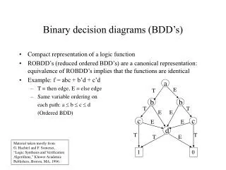
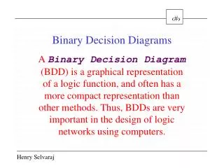
Binary Decision Diagrams. A Binary Decision Diagram (BDD) is a graphical representation of a logic function, and often has a more compact representation than other methods. Thus, BDDs are very important in the design of logic networks using computers. A. B. C. 1. 1. 0. 0. Example. 0.

Binary Decision Diagrams
E N D
Presentation Transcript
Binary Decision Diagrams A Binary Decision Diagram (BDD) is a graphical representation of a logic function, and often has a more compact representation than other methods. Thus, BDDs are very important in the design of logic networks using computers.
A B C 1 1 0 0 Example 0 1 0 1 F = A + BC’ If A = 1 , then f = 1 Let A = 0, if B = 0, then f = 0. Let A = 0, if B = 1, if C = 1 then f = 0 Let A = 0, if B = 1, if C = 0 then f = 1 1 0
In general, the complete binary decision tree for an n-variable function has 2n different paths, and there is one-to-one correspondence between the terminal nodes of BDDs and 2n elements of the truth table. The total number of nodes is 2n+1 -1
Binary Decision Diagrams (BDDs) BDDs are canonical, so if you correctly build the BDDs for two circuits, the two circuits are equivalent if and only if the BDDs are identical. This has led to significant breakthroughs in circuit optimization, testing and equivalence checking.
BDDs are very effective in representing combinatorially large sets. This has led to breakthroughs in FSM (Finite State Machines) equivalence checking and in two level logic minimization.
Difficulties with SOP and POS representation EXOR representation is too big Changing from SOP to POS & vice versa is difficult (..therefore, taking complement is difficult Taking AND of two SOP or OR of tro POS is hard. they
3 3 2 0 1 2 1 0 1 1 0 1 0 1 0 0 1 1 0
a b 1 0 1 f = a . b 0 1 0
a b 0 1 0 f = a + b 1 0 1
1 2 2 3 3 0 1 0 1 0 1 1 1 0 0 0 1 1 0
Isomorphism between OBDDs Two OBDDs G1 and G2 are isomorphic if there exists a one-to-one function σ from the vertices of G1 onto the vertices of G2 such that for any vertex v if σ(v) = w, then either both v and w are terminal vertices with value (v) = value (w), or both v and w are nonterminal vertices with index (v) = index (w), σ (low (v)) = low (w) and σ (high (v)) = high (w)
Every function is represented by a unique ROBDD for a given ordering of inputs to the function.
1 2 3 3 2 1 0 1 0 1 Compliment 0 0 1 1 1 1 0 0 1 1
Complementing an ROBDD can be trivially accomplished by Interchanging the 0 and 1 terminal vertices.
Artificial Neural Networks Artificial Neural Networks (ANNs) is an abstract simulation of a real nervous system that contains a collection of neuron units communicating with each other via axon connections. Such a model bears a strong resemblance to axons and dendrites in a nervous system. The first fundamental modeling of neural nets was proposed in 1943 by McCulloch and Pitts in terms of a computational model of "nervous activity".
The first is the biological type. It encompasses networks mimicking biological neural systems such as audio functions or early vision functions. The other type is application-driven. It depens less on the faithfulness to neurobiology. For these models the architectures are largely dictated by the application needs. Many such neural networks are represented by the so called connectionist models. Types of ANN
Neurons and the interconnection synapses constitute the key elements for neural information processing.
It is estimated that the human brain contains over 100 billion neurons and synapses in the human nervous system. Studies of brain anatomy of the neurons indicate more than 1000 synapses on the input and output of each neuron. Note that, although the neuron's switch time (a few milliseconds) is about a million fold times slower than current computer elements, they have a thousand fold greater connectivity than today’s supercomputers.
a neuron cell body, branching extensions called dendrites for receiving input, and an axon that carries the neuron's output to the dendrites of other neurons. Three parts of a neuron
A neuron collects signals at its synapses by summing all the excitatory and inhibitory influences acting on it. If the excitatory influences are dominant, then the neuron fires and sends this message to other neurons via the outgoing synapses. In this sense, the neuron function can be modeled as a simple threshold function f(.). The neuron fires if the combined signal strength exceeds a certain threshold value. activation function f(.)
The strength of application-driven neural networks hinges upon three main characteristics: Adaptiveness and self-organization: it offers robust and adaptive processing capabilities by adopting adaptive learning and self-organization rules. Nonlinear network processing: it enhances the network's approximation, classification and noise-immunity capabilities. Parallel processing: it usually employs a large number of processing cells enhanced by extensive interconnectivity. Application-Driven Neural Networks
An engineering approach • An artificial neuron is a device with many inputs and one output. The neuron has two modes of operation; the training mode and the using mode. In the training mode, the neuron can be trained to fire (or not), for particular input patterns. In the using mode, when a taught input pattern is detected at the input, its associated output becomes the current output. If the input pattern does not belong in the taught list of input patterns, the firing rule is used to determine whether to fire or not.
A simple firing rule can be implemented by using Hamming distance technique: Take a collection of training patterns for a node, some of which cause it to fire (the 1-taught set of patterns) and others which prevent it from doing so (the 0-taught set). Then the patterns not in the collection cause the node to fire if, on comparison , they have more input elements in common with the 'nearest' pattern in the 1-taught set than with the 'nearest' pattern in the 0-taught set. If there is a tie, then the pattern remains in the undefined state. Firing rules
Example • A 3-input neuron is taught to output 1 when the input (X1,X2 and X3) is 111 or 101 and to output 0 when the input is 000 or 001. Then, before applying the firing rule, the truth table is:
The architecture of a Perceptron consists of a single input layer of many neurodes, and a single output layer of many neurodes. The simple "networks" illustrated at the beginning, to produce logical "AND" and "OR" operations have a Perceptron architecture. But to be called a Perceptron, the network must also implement the Perceptron learning rule for weight adjustment. PERCEPTRONS
In Backprop, a third neurode layer is added (the hidden layer) and the discrete thresholding function is replaced with a continuous (sigmoid) one. But the most important modification for Backprop is the generalized delta rule, which allows for adjustment of weights leading to the hidden layer neurodes in addition to the usual adjustments to the weights leading to the output layer neurodes. Using the generalize delta rule to adjust the weights leading to the hidden units is backpropagating the error-adjustment.
a. Each unit in the network has connections to other units in the network. Each connection from unit i to unit j is weighted with weight W(i,j). b. Each unit requires an activation function which takes as input the sum of all inputs into the unit (weighted by their respective weights). The output of the activation function is usually a value between 1 and 0 (unit fires/ doesnt fire). The step function is used a lot in multilayer networks but for back propagation we will have to determine the derivative of the activation function so that will not work. Sigmoid is a better activation function and its derivate is relatively simple. Sigmoid(x) = 1/(1+e(-x)) Backprob
a. To do back propagation we take a network with arbitrary weights to start and we begin by applying one of our training examples to the network. We calculate network all the way to the output. b. Once we have an output we calculate the Err(i) vector representing the error between our desired value and the actual output. Method of Back Propagation
c. Then for each output unit i we update the weights of the connections from Unit j to the unit i as so: W(j,i) = W(j,i) + *ai * err(i) * g(input(i)) Where ai = the output of i. Input(i) = the sum of all inputs to unit(i) weighted appropriately g = the derivative of the activation function of unit(i) err(i) = the error defined above = the learning constant (passed as a parameter to the supervised learning algorithm. All this does is control how much of the error is taken into consideration when we update the weight. For example =0.1 will not change W(j,i) as much as =0.5).
After we update all the weights to the output layer of the network we can propagate the error back a layer. The error for a unit(j) in this layer is just the sum of all the errors of the units(i) that unit(j) connects to weighted by the weight of the connection. So, err(j) = W(j,i)*err(i) (And now we can update the weights connecting to unit(j) just as before).
e. Next we repeatedly propagate the error back using equation 1 until all weights have been updated. f. Now that we have updated the network to this training example we can start over and apply another training example. We should repeat examples over and over again until the weights of the network converge.