Download
1 / 37
370 likes | 387 Views
This course module explores decision theory, including single and sequential decision problems, representation and reasoning techniques, and stochastic and deterministic problem types.

E N D
Decision Theory: Single & Sequential Decisions. VE for Decision Networks. CPSC 322 – Decision Theory 2 Textbook §9.2 April 1, 2011
Course Overview Course Module Representation Environment Reasoning Technique Stochastic Deterministic Problem Type Arc Consistency Constraint Satisfaction Decision theory:acting under uncertainty Variables + Constraints Search Static Bayesian Networks Logics Logic Uncertainty Search Variable Elimination Decision Networks Sequential STRIPS Search Variable Elimination Decision Theory Planning Planning As CSP (using arc consistency) Markov Processes Value Iteration
Lecture Overview • Recap: Utility and Expected Utility • Single-Stage Decision Problems • Single-Stage decision networks • Variable elimination (VE) for computing the optimal decision • Sequential Decision Problems • General decision networks • Time-permitting: Policies • Next lecture: variable elimination for finding the optimal policy in general decision networks
Utility • Utility: a measure of desirability of possible worlds to an agent • Let U be a real-valued function such that U(w) represents an agent's degree of preference for world w • Simple goals can still be specified: e.g. • Worlds that satisfy the goal have utility 100 • Other worlds have utility 0 • Utilities can be more complicated • For example, in the robot delivery domains, they could involve • Amount of damage • Reached the target room? • Energy left • Time taken
Delivery Robot Example • Decision variable 1: the robot can choose to wear pads • Yes: protection against accidents, but extra weight • No: fast, but no protection • Decision variable 2: the robot can choose the way • Short way: quick, but higher chance of accident • Long way: safe, but slow • Random variable: is there an accident? Utility Agent decides 35 95 Chance decides 30 75 3 35 100 0 35 80
Possible worlds and decision variables • A possible world specifies a valuefor each random variable and each decision variable • For each assignment of values to all decision variables • the probabilities of the worlds satisfying that assignment sum to 1. Conditional probability Utility 0.2 35 35 95 0.8 35 30 0.01 75 0.99 0.2 35 3 100 0.8 35 0 0.01 80 0.99
Expected utility of a decision Conditional probability Utility E[U|D] 0.2 35 35 83 95 0.8 35 30 0.01 74.55 75 0.99 0.2 35 3 80.6 100 0.8 35 0 0.01 79.2 80 0.99
Lecture Overview • Recap: Utility and Expected Utility • Single-Stage Decision Problems • Single-Stage decision networks • Variable elimination (VE) for computing the optimal decision • Sequential Decision Problems • General decision networks • Time-permitting: Policies • Next lecture: variable elimination for finding the optimal policy in general decision networks
Single Action vs. Sequence of Actions • Single Action (aka One-Off Decisions) • One or more primitive decisions that can be treated as a single macro decision to be made before acting • E.g., “WearPads” and “WhichWay” can be combined into macro decision (WearPads, WhichWay) with domain {yes,no} × {long, short} • Sequence of Actions (Sequential Decisions) • Repeat: • make observations • decide on an action • carry out the action • Agent has to take actions not knowing what the future brings • This is fundamentally different from everything we’ve seen so far • Planning was sequential, but we still could still think first and then act
Optimal single-stage decision • Given a single (macro) decision variable D • the agent can choose D=difor any value di dom(D)
What is the optimal decision in the example? Conditional probability (Wear pads, short way) Utility E[U|D] (Wear pads, long way) 0.2 35 35 (No pads, short way) 83 95 0.8 (No pads, long way) 30 35 0.01 74.55 75 0.99 0.2 35 3 80.6 100 0.8 35 0 0.01 79.2 80 0.99
Optimal decision in robot delivery example Best decision: (wear pads, short way) Conditional probability Utility E[U|D] 0.2 35 35 83 95 0.8 30 35 0.01 74.55 75 0.99 0.2 35 3 80.6 100 0.8 35 0 0.01 79.2 80 0.99
Single-Stage decision networks • Extend belief networks with: • Decision nodes, that the agent chooses the value for • Parents: only other decision nodes allowed • Domain is the set of possible actions • Drawn as a rectangle • Exactly one utility node • Parents: all random & decision variables on which the utility depends • Does not have a domain • Drawn as a diamond • Explicitly shows dependencies • E.g., which variables affect the probability of an accident?
Types of nodes in decision networks • A random variable is drawn as an ellipse. • Arcs into the node represent probabilistic dependence • As in Bayesian networks: a random variable is conditionally independent of its non-descendants given its parents • A decision variable is drawn as an rectangle. • Arcs into the node represent information available when the decision is made • A utility node is drawn as a diamond. • Arcs into the node represent variables that the utility depends on. • Specifies a utility for each instantiation of its parents
Example Decision Network Decision nodes do not have an associated table. The utility node does not have a domain.
Computing the optimal decision: we can use VE • Denote • the random variables as X1, …, Xn • the decision variables as D • the parents of node N as pa(N) • To find the optimal decision we can use VE: • Create a factor for each conditional probability and for the utility • Sum out all random variables, one at a time • This creates a factor on D that gives the expected utility for each di • Choose the diwith the maximum value in the factor
VE Example: Step 1, create initial factors f1(A,W) Abbreviations: W = Which WayP = Wear PadsA = Accident f2(A,W,P)
VE example: step 2, sum out A Step 2a: compute product f1(A,W) × f2(A,W,P) What is the right form for the product f1(A,W) × f2(A,W,P)? f(A,W) f(A,P) f(A) f(A,P,W)
VE example: step 2, sum out A Step 2a: compute product f(A,W,P) = f1(A,W) × f2(A,W,P) What is the right form for the product f1(A,W) × f2(A,W,P)? • It is f(A,P,W): the domain of the product is the union of the multiplicands’ domains • f(A,P,W) = f1(A,W) × f2(A,W,P) • I.e., f(A=a,P=p,W=w) = f1(A=a,W=w) × f2(A=a,W=w,P=p)
VE example: step 2, sum out A Step 2a: compute product f(A,W,P) = f1(A,W) × f2(A,W,P) f(A=a,P=p,W=w) = f1(A=a,W=w) × f2(A=a,W=w,P=p) 0.99 * 30 0.01 * 80 0.99 * 80 0.8 * 30
VE example: step 2, sum out A Step 2a: compute product f(A,W,P) = f1(A,W) × f2(A,W,P) f(A=a,P=p,W=w) = f1(A=a,W=w) × f2(A=a,W=w,P=p)
VE example: step 2, sum out A Step 2b: sum A out of the product f(A,W,P): 0.2*35 + 0.2*0.3 0.2*35 + 0.8*95 0.99*80 + 0.8*95 0.8 * 95 + 0.8*100
VE example: step 2, sum out A Step 2b: sum A out of the product f(A,W,P):
VE example: step 3, choose decision with max E(U) The final factor encodes the expected utility of each decision • Thus, taking the short way but wearing pads is the best choice, with an expected utility of 83 Step 2b: sum A out of the product f(A,W,P):
Variable Elimination for Single-Stage Decision Networks: Summary • Create a factor for each conditional probability and for the utility • Sum out all random variables, one at a time • This creates a factor on D that gives the expected utility for each di • Choose the di with the maximum value in the factor
Lecture Overview • Recap: Utility and Expected Utility • Single-Stage Decision Problems • Single-Stage decision networks • Variable elimination (VE) for computing the optimal decision • Sequential Decision Problems • General decision networks and Policies • Next lecture: variable elimination for finding the optimal policy in general decision networks
Sequential Decision Problems • An intelligent agent doesn't make a multi-step decision and carry it out blindly • It would take new observations it makes into account • A more typical scenario: • The agent observes, acts, observes, acts, … • Subsequent actions can depend on what is observed • What is observed often depends on previous actions • Often the sole reason for carrying out an action is to provide information for future actions • For example: diagnostic tests, spying • General Decision networks: • Just like single-stage decision networks, with one exception:the parents of decision nodes can include random variables
Sequential Decision Problems: Example • Example for sequential decision problem • Treatment dependson Test Result (& others) • Each decision Di has an information set of variables pa(Di), whose value will be known at the time decision Di is made • pa(Test) = {Symptoms} • pa(Treatment) = {Test, Symptoms, TestResult} Decision node: Agent decides Chance node: Chance decides
Sequential Decision Problems: Example • Another example for sequential decision problems • Call depends onReport and SeeSmoke(and on CheckSmoke) Decision node: Agent decides Chance node: Chance decides
Sequential Decision Problems • What should an agent do? • What an agent should do depends on what it will do in the future • E.g. agent only needs to check for smoke if that will affect whether it calls • What an agent does in the future depends on what it did before • E.g. when making the decision it needs to whether it checked for smoke • We will get around this problem as follows • The agent has a conditional plan of what it will do in the future • We will formalize this conditional plan as a policy
Policies for Sequential Decision Problems Definition (Policy)A policy is a sequence of δ1 ,…..,δn decision functions δi : dom(pa(Di )) → dom(Di) This policy means that when the agent has observed odom(pDi) , it will do δi(o) • There are 22=4 possible decision functions δcsfor Check Smoke: • Decision function needs to specify a value for each instantiation of parents CheckSmoke Call
Policies for Sequential Decision Problems Definition (Policy)A policy is a sequence of δ1 ,…..,δn decision functions δi : dom(pa(Di )) → dom(Di) • There are 28=256 possible decision functions δcsfor Call: • Decision function needs to specify a value for each instantiation of parents Call ……
How many policies are there? • If a decision D has k binary parents, how many assignments of values to the parents are there? 2k 2+k k2 2k
How many policies are there? • If a decision D has k binary parents, how many assignments of values to the parents are there? • 2k • If there are b possible value for a decision variable, how many different decision functions are there for it if it has k binary parents? • 2kp • b*2k • b2k • 2kb
How many policies are there? • If a decision D has k binary parents, how many assignments of values to the parents are there? • 2k • If there are b possible value for a decision variable, how many different decision functions are there for it if it has k binary parents? • b2k
Learning Goals For Today’s Class • Compare and contrast stochastic single-stage (one-off) decisions vs. multistage decisions • Define a Utility Function on possible worlds • Define and compute optimal one-off decisions • Represent one-off decisions as single stage decision networks • Compute optimal decisions by Variable Elimination • Next time: • Variable Elimination for finding optimal policies
Announcements • Assignment 4 is due on Monday • Final exam is on Monday, April 11 • The list of short questions is online … please use it! • Office hours next week • Simona: Tuesday, 10-12 (no office hours on Monday!) • Mike: Wednesday 1-2pm, Friday 10-12am • Vasanth: Thursday, 3-5pm • Frank: • X530: Tue 5-6pm, Thu 11-12am • DMP 110: 1 hour after each lecture • Optional Rainbow Robot tournament: Friday, April 8 • Hopefully in normal classroom (DMP 110) • Vasanth will run the tournament, I’ll do office hours in the same room (this is 3 days before the final)