Download
1 / 25
260 likes | 361 Views
Learn how to implement a Lag Compensator Control to the physical system using Simulink. Follow the steps to re-write the final equation of motion and observe the closed-loop response.

E N D
The final simulink model now is shown below. See how you can change some aspects but get the same effect.
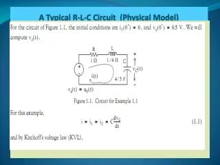
Implementing Lag Compensator Control • In the motor speed control root locus example a Lag Compensator was designed with the following transfer function. • To implement this in Simulink, we will contain the open-loop system from earlier in this page in a Subsystem block. • Create a new model window in Simulink. • Drag a Subsystem block from the Connections block library into your new model window.
Double click on this block. You will see a blank window representing the contents of the subsystem (which is currently empty). • Open your previously saved model of the Motor Speed system, motormod.mdl. • Select All from the Edit menu (or Ctrl-A), and select Copy from the Edit menu. Select the blank subsystem window from your new model and select Paste from the Edit menu (or Ctrl-V). You should see your original system in this new subsystem window. Close this window.
You should now see input and output terminals on the Subsystem block. • Name this block "plant model". • Now, we will insert a Lag Compensator into a closed-loop around the plant model. • First, we will feed back the plant output. • Draw a line extending from the plant output. • Insert a Sum block and assign "+-" to it's inputs. • Tap a line of the output line and draw it to the negative input of the Sum block.
The output of the Sum block will provide the error signal. • We will feed this into a Lag Compensator. • Insert a Transfer Function Block after the sum and connect them with a line. • Edit this block and change the Numerator field to • "[50 50]" and the denominator field to • "[1 0.01]". • Label this block "Lag Compensator“ as seen on the next slide.
Finally, we will apply a step input and view the output on a scope. • Attach a step block to the free input of the feedback Sum block and attach a Scope block to the plant output. • Double-click the Step block and set the Step Time to "0".
Closed-loop response • To simulate this system, first, an appropriate simulation time must be set. • Select Parameters from the Simulation menu and enter "3" in the Stop Time field. • The design requirements included a settling time of less than 2 sec, so we simulate for 3 sec to view the output. • The physical parameters must now be set. Run the following commands at the MATLAB prompt: J=0.01; b=0.1; K=0.01; R=1; L=0.5; • Run the simulation (Start on the Simulation menu). When the simulation is finished, double-click on the scope and hit its auto-scale button. You should see the following output.