Download
1 / 47
510 likes | 792 Views
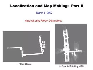
Maps built using Parker’s DILab robots:. Localization and Map Making: Part II. March 8, 2007. 1 st Floor Claxton. 1 st Floor, JICS Building, ORNL. The Player/Stage “Localize” Proxy. Allows you to localize the robot using its sensors (e.g., laser or sonar, or even radio strength of signal).

E N D
Maps built using Parker’s DILab robots: Localization and Map Making: Part II March 8, 2007 1st Floor Claxton 1st Floor, JICS Building, ORNL
The Player/Stage “Localize” Proxy • Allows you to localize the robot using its sensors (e.g., laser or sonar, or even radio strength of signal) Public Member Functions: LocalizeProxy (PlayerClient *aPc, uint aIndex=0) constructor ~LocalizeProxy () destructor uint GetMapSizeX () const Map dimensions (cells). uint GetMapSizeY () const uint GetMapTileX () const uint GetMapTileY () const double GetMapScale () const Map scale (m/cell). uint GetPendingCount () const # of pending (unprocessed) sensor readings. uint GetHypothCount () const Number of possible poses.player_localize_hypoth_tGetHypoth (uint aIndex) const Array of possible poses. int GetParticles () Get the particle set. player_pose_tGetParticlePose (int index) const Get the Pose of a particle. void SetPose (double pose[3], double cov[3]) Set the current pose hypothesis (m, m, radians). uint GetNumHypoths () const Get the number of localization hypotheses uint GetNumParticles () const Get # of particles (for particle filter-based localization systems).
Player/Stage Localization Approach:Monte Carlo Localization • Based on techniques developed by Fox, Burgard, Dellaert, Thrun (see handout of AAAI’99 article) (Movie illustrating approach)
Two types of localization problems • “Global” localization – figure out where the robot is, but we don’t know where the robot started • Sometimes called the “hijacked robot problem” • “Position tracking” – figure out where the robot is, given that we know where the robot started The Monte Carlo Localization approach of Fox, et al (which is in Player/Stage) can address both problems
Markov Localization • Key idea: compute a probability distribution over all possible positions in the environment. • This probability distribution represents the likelihood that the robot is in a particular location. P(Robot Location) Y State space = 2D, infinite #states X Slide adapted from Dellaert presentation “19-Particles.ppt”
Side note: What does “Markov” mean? • “Markov” means the system obeys the “Markov Property” • “Markov Property”: the conditional probability of the future state is dependent only on the current state. It is independent of the past states. • For the purposes of robot localization • Future sensor readings are conditionally independent of past readings, given the true current position of the robot. • Means we don’t have to save all the prior sensor data and apply it each time we update beliefs on the robot’s location.
Markov Localization (con’t.) • Let l = <x, y, > represent a robot position in space • Bel(l) represents the robot’s belief that it is at position l • Bel(l) is a probability distribution, centered on the correct position • As the robot moves, Bel(l) is updated • Two probabilistic models used to update Bel(l) • Action (or motion) model: represents movements of robot • Perception (or sensing) model: represents likelihood that robot senses a particular reading at a particular position (related to our discussion last class) “Probability that an action a in position l moves the robot to position l, times the likelihood the robot is in positionl , integrated over all possible ways robot could have reached position l” “Probability that robot will perceive s, given that the robot is in position l, times the likelihood the robot is in positionl”
sensor motion motion Can implement Markov Localization in different ways Very commonly used approach: • Kalman Filter – estimates state from a series of incomplete, noisy measurements (e.g., sensor readings) • At each point in time, a new estimate of robot’s position is made, using action (sometimes called “motion”) model and sensor model • Maintains a single estimate of robot’s position (Also, other Markov Localization approaches we won’t go into here…) Slide adapted from Dellaert presentation “19-Particles.ppt”
Different Concept for implementing Markov Localization: Monte Carlo Localization using Particle Filtering • Maintain multiple estimates of robot’s location • Track possible robot positions, given all previous measurements • Key idea: represent the belief that a robot is at a particular location by a set of “samples”, or “particles” Represent Bel(l) by set of N weighted, random samples, called particles: where a sample, si, is of the form: <<x, y, >, p> Here, <x, y, > represents robot’s position (just like before) p represents a weight, where sum of all p’s is 1 (analogous to discrete probability)
Side Note: What does “Monte Carlo” mean? • Refers to techniques that are stochastic / random / non-deterministic • Used in lots of modeling and simulation approaches • Particularly useful when the system has significant uncertainty in the inputs (e.g., robot localization!)
Updating beliefs using Monte Carlo Localization (MCL) • As before, 2 models: Action (Motion) Model, Perception (Sensing) Model • Robot Motion Model: • When robot moves, MCL generates N new samples that approximate robot’s position after motion command. • Each sample is generated by randomly drawing from previous sample set, with likelihood determined by p values. • For sample drawn with position l, new sample l is generated from P(l | l, a) • p value of new sample is 1/N Sampling-based approximation of position belief for non-sensing robot (From Fox, et al, AAAI-99)
Updating beliefs using Monte Carlo Localization (MCL) (con’t.) • Robot Sensing Model: • Re-weight sample set, according to the likelihood that robot’s current sensors match what would be seen at a given location • Let < l, p> be a sample. • Then, p P(s | l) Here, s is the sensor measurement; a normalization constant to enforce the sum of p’s equaling 1 • After applying Motion model and Sensing model: • Resample, according to latest weights • Add a few uniformly distributed, random samples • Very helpful in case robot completely loses track of its location
s <x,y,>t Side Note: Common Terminology • Prediction Phase: Applying motion model • Measurement Phase: Applying sensor model <x,y,>t-1 <x,y,>t Slide adapted from Dellaert presentation “19-Particles.ppt”
Adapting the Size of the Sample Set • Number of samples needed to achieve a desired level of accuracy varies dramatically depending on the situation • During global localization: robot is ignorant of where it is need lots of samples • During position tracking: robot’s uncertainty is small don’t need as many samples • MCL determines sample size “on the fly” • Compare P(l) and P(l | s) (I.e., belief before and after sensing) to determine sample size • The more divergence, the more samples that are kept
What sensor to use for localization? • Can work with: • Sonar • Laser • Vision • Radio signal strength
Example Results Initially, robot doesn’t know where it is (see particles representing possible robot locations distributed throughout the environment) After robot moves some, it gets better estimate (see particles clustered an a few areas, with a few random particles also distributed around for robustness)
More movies • Dieter Fox movie: MCL using Sonar • Dieter Fox movie: MCL using Laser
Summarizing the process: Particle Filtering St-1 weighted S’t St S’t Predict Resample ReWeight Slide adapted from Dellaert presentation “19-Particles.ppt”
Mapping is much easier if robot can localize • SLAM: Simultaneous Localization And Mapping • If robot knows where it is, then it can merge its sensor measurements as it moves, effectively building a map • But, lots of details, like “closing the loop” in maps that are very important, and challenging • “Closing the loop”: splicing together pieces of the map that represent the same part of the environment, but which are explored by robot at different times • We won’t go into details here… Example:
Case Study: A Different Approach to Multi-Robot Localization • Work at University of Southern California • SLAM (Simultaneous Localization and Mapping) • Relaxation on a mesh • Maximum likelihood estimation • Scenario modeled with: • The Stage simulator • Multi-operator, multi-robot tasking
Localization • Past approaches include: • Filtering inertial sensors for location estimation • Using landmarks (based on vision, laser etc.) • Using maps • Algorithms vary from Kalman filters, to Markov localization to Particle filters • This case study approach • Exploit communication for in-network localization • Physics-based models
Static Localization • System contains beacons and beacon detectors • Assumptions: • beacons are unique, • beacon detectors determine correct identity. • Static localization: • determine the relative pose of each pair of beacons/detectors
Mesh Energy Kinetic energy Potential energy
Mesh Forces and Equations of Motion Forces Equations of motion
SLAM: Simultaneous Localization and Mapping Localization
Multi-robot SLAM Localization
Team Localization using MLE • Construct a set of estimates H = {h} where h is the pose of robot r at time t. • Construct a set of observations O = {o} where o is either: the measured pose of robot rb relative to robot ra at time t, or the measured change in pose of robot r between times ta and tb. • Assuming statistical independence between observations find the set of estimates H that maximizes:
Approach Equivalently, find the set H that minimizes:
Gradient-based Estimation • Each estimate • Each observation • Measurement uncertainty assumed normal • Relative Absolute
Gradient Descent • Compute set of poses q that minimizes U(O|H) • Gradient-based algorithm
Range Error vs. Time Robots bump into each other
Summary of USC Team Localization Approach • Runs on any platform as long as it can compute its motion via inertial sensing • Unique beacons: robots, people, fixed locations etc. • No model of the environment • Indifferent to changes in the environment • Robust to sensor noise • Permits both centralized and distributed implementation
Overall Localization and Map Making Picture D E R I V E D M A P A C T U A T O R S motor commands Exploration Map Update Recent Motor Command History S E N S O R S x,y prob. distribution Localization expected sensory changes
Exploration • Key question: Where hasn’t robot been? • Central concern: how to cover an unknown area efficiently • Possible approaches: • Random walk • Use proprioception to avoid areas that have been recently visited • Exploit evidential information in the occupancy grid • Two basic styles of exploration: • Frontier-based • Generalized Voronoi graph
Frontier-Based Exploration • Assumes robots uses Bayesian occupancy grid • When robot enters new area, find boundary (“Frontier”) between sensed (and open) and unsensed areas • Head towards centroid of Frontier Robot’s current position Frontier Centroid of frontier Frontier
Calculating Centroid • Centroid is average (x,y) location: x_c = y+c = count = 0 for every cell on the frontier line with a location of (x,y) { x_c = x_c + x y_c = y_c + y count++ } x_c = x_c/count y_c = y_c/count
Motion Control Based on Frontier Exploration • Robot calculates centroid • Robot navigates using: • Move-to-goal and avoid-obstacle behaviors • Or, plan path and reactively execute the path • Or, continuously replan and execute the path • Once robot reaches frontier, map is updated and new frontiers (perhaps) discovered • Continue until no new frontiers remaining
Movie of Frontier-Based Exploration • (from Dieter Fox)
Generalized Voronoi Graph Methods of Exploration • Robot builds reduced generalized Voronoi graph (CVG) as it moves through world • As robot moves, it attempts to maintain a path that is equidistant from all objects it senses (called “CVG edge”) • When robot comes to gateway, randomly choose branch to follow, remembering the other edge(s) • When one path completely explored, backtrack to previously detected branch point • Exploration and backtracking continue until entire area covered.
Summary of Localization and Map Making • Map-making: converts local sensor observations into global map, independent of robot position • Most common data structure for mapping: occupancy grid • Occupancy grid: 2D array, representing fixed area • Use probabilistic sensor models and Bayesian methods to update occupancy grid based upon multiple observations • Producing global map requires localization • Raw sensory data (especially odometry) is imperfect • Two types of localization: iconic, feature-based • Two types of formal exploration strategies: frontier-based and CVG