Download
1 / 31
340 likes | 713 Views
Properties of Poisson. The mean and variance are both equal to . The sum of independent Poisson variables is a further Poisson variable with mean equal to the sum of the individual means. The Poisson distribution provides an approximation for the Binomial distribution. Approximation:

E N D
Properties of Poisson The mean and variance are both equal to . The sum of independent Poisson variables is a further Poisson variable with mean equal to the sum of the individual means. The Poisson distribution provides an approximation for the Binomial distribution.
Approximation: If n is large and p is small, then the Binomial distribution with parameters n and p is well approximated by the Poisson distribution with parameter np, i.e. by the Poisson distribution with the same mean
Example Binomial situation, n= 100, p=0.075 Calculate the probability of fewer than 10 successes.
> pbinom(9,100,0.075) [1] 0.7832687 > This would have been very tricky with manual calculation as the factorials are very large and the probabilities very small
The Poisson approximation to the Binomial states that will be equal to np, i.e. 100 x 0.075 so =7.5 > ppois(9,7.5) [1] 0.7764076 > So it is correct to 2 decimal places. Manually, this would have been much simpler to do than the Binomial.
Poisson Approximation: the Birthday Problem. What is the probability that in a gathering of k people, at least two share the same birthday?
Suppose there are n days in the year (on Earth we have n = 365) Assume that each person has a birthday which is equally likely to fall on any day of the year, independently of the birthdays of the remaining k - 1 persons (no sets of twins in the group).
Then a simple conditional probability calculation shows that pn;k = 1- p(all birthdays are different) = We can write a simple R function - call it probcoincide - to evaluate pn;k for any n and k
> probcoincide = function(n,k) 1 - prod((n-1):(n-k+1))/n^(k-1)
> probcoincide = function(n,k) 1 - prod((n-1):(n-k+1))/n^(k-1) > probcoincide(365,22) [1] 0.4756953 >
> probcoincide = function(n,k) 1 - prod((n-1):(n-k+1))/n^(k-1) > probcoincide(365,23) [1] 0.5072972 >
So that (on Earth) 23 is the minimum size of gathering required for a better than evens chance of two members sharing the same birthday. Proof of this The mean number of birthday coincidences in a sample of size k is:
The number of birthday coincidences should have an approximately Poisson distribution with the above mean. Thus, to determine the size of gathering required for an approximate probability p of at least one coincidence, we should solve
In other words we are solving the simple quadratic equation In the case n=365, p=0.5, this gives k=23.0
Simulation with Poisson Just like in the case for Binomial, Poisson results can be simulated in R. (rpois) Example Simulate 500 occurrences of arrivals at a bus-stop in a 1 hour period if the distribution is Poisson with mean 5.3 per hour.
> ysim=rpois(500,5.3) > ysim [1] 6 10 8 4 6 1 2 4 6 9 8 3 5 5 3 7 6 6 3 6 6 4 9 6 3 [26] 6 6 4 4 3 3 5 8 4 10 6 6 5 5 5 5 3 3 10 6 5 3 7 3 3 [51] 6 4 5 6 5 5 7 8 3 4 8 5 6 5 3 2 3 3 3 5 3 8 8 4 5 [76] 3 3 3 8 7 9 3 3 8 9 7 8 3 4 1 5 9 1 6 5 8 3 7 4 7 [101] 1 8 8 6 5 3 4 0 7 4 7 5 7 6 7 4 7 6 1 3 8 9 5 5 10 [126] 4 6 5 6 8 3 8 4 5 9 8 7 4 2 3 6 6 6 6 4 3 6 11 4 7 [151] 4 3 9 4 3 3 5 7 13 5 7 1 10 6 5 4 6 7 9 9 4 5 7 9 8 [176] 6 7 6 4 6 11 3 6 8 3 6 2 1 8 7 8 6 4 4 4 6 4 3 2 7 [201] 5 6 7 6 7 6 9 7 3 7 6 8 3 5 2 9 6 6 8 3 6 5 2 3 7 [226] 2 6 11 5 5 4 5 7 8 3 5 8 2 7 5 3 6 5 9 1 5 8 8 6 6 [251] 5 10 5 4 7 6 8 2 6 1 5 5 7 3 0 2 7 7 10 4 6 6 4 5 8 [276] 7 3 7 6 3 5 7 6 4 4 0 2 5 5 4 5 5 6 5 5 7 7 7 8 7 [301] 9 2 8 5 12 3 10 5 5 8 3 5 3 6 5 8 4 7 3 3 4 6 2 1 2 [326] 6 7 3 2 3 8 4 7 3 6 5 4 5 7 7 7 4 7 6 4 5 3 4 2 8 [351] 7 5 5 6 6 6 7 9 11 4 3 4 9 6 9 4 1 3 7 2 6 1 2 9 5 [376] 7 6 3 7 7 5 5 6 4 6 9 5 8 10 3 8 6 4 7 6 3 6 6 4 2 [401] 3 3 6 5 7 4 4 5 8 8 5 12 9 14 3 12 3 2 5 4 5 7 7 3 7 [426] 7 9 7 4 7 5 2 6 5 6 8 5 3 8 4 7 4 4 5 3 4 6 3 6 6 [451] 7 7 3 6 2 7 6 9 4 9 11 4 6 3 1 3 7 9 8 4 4 10 9 7 10 [476] 2 3 6 4 6 6 8 3 12 6 6 3 4 3 0 3 7 6 7 6 3 3 1 2 4
A table of the results is constructed > table(ysim) ysim 0 1 2 3 4 5 6 7 8 9 10 11 12 13 14 4 14 25 76 63 72 87 68 43 26 11 5 4 1 1 >
Poisson distributions have expected value and variance both equal to . Check this out for our simulations. > mean(ysim) [1] 5.44 > var(ysim) [1] 5.565531 >
Both are slightly out so see what happens if we simulate 5000 observations rather than 500. > ysim=rpois(5000,5.3) > mean(ysim) [1] 5.3502 > var(ysim) [1] 5.141388 >
And for 50 000 > ysim=rpois(50000,5.3) > mean(ysim) [1] 5.29968 > var(ysim) [1] 5.335299 >
R is built from packages of datasets and functions. The base and ctest packages are loaded by default and contain everything necessary for basic statistical analysis. Other packages may be loaded on demand, either via the Packages menu, or via the R function library.
Once a package is loaded, the functions within it are automatically available. To make available a dataset from within a package, use the function data. Of particular interest to advanced statistical users is the package MASS, which contains the functions and datasets from the book Modern Applied Statistics with S by W N Venables and B D Ripley. This package can be loaded with > library(MASS)
To make available the dataset chemfrom within MASS, use additionally > data(chem) Documentation on any package is available via the R help system. Missing or further packages may usually be obtained from CRAN.
Some data sets are already in R when you open it. > data(iris) > iris Sepal.Length Sepal.Width Petal.Length Petal.Width Species 1 5.1 3.5 1.4 0.2 setosa 2 4.9 3.0 1.4 0.2 setosa 3 4.7 3.2 1.3 0.2 setosa 4 4.6 3.1 1.5 0.2 setosa 5 5.0 3.6 1.4 0.2 setosa 6 5.4 3.9 1.7 0.4 setosa 7 4.6 3.4 1.4 0.3 setosa 8 5.0 3.4 1.5 0.2 setosa 9 4.4 2.9 1.4 0.2 setosa 10 4.9 3.1 1.5 0.1 setosa
Notice, though, that if you haven’t used the data command, R will not know that iris exists. Type `demo()' for some demos, `help()' for on-line help, or `help.start()' for a HTML browser interface to help. Type `q()' to quit R. [Previously saved workspace restored] > iris Error: Object "iris" not found >
Similarly if you use a file from the library and do not use the library command first, R will not know that a data set exists. Type `demo()' for some demos, `help()' for on-line help, or `help.start()' for a HTML browser interface to help. Type `q()' to quit R. [Previously saved workspace restored] > data(chem) Warning message: Data set `chem' not found in: data(chem) >