Download
1 / 1
10 likes | 81 Views
Explore non-invasive monitoring & control in ultrasound therapy. Study temperature profiles and challenges faced in ultrasound images. Gather data from gelatine phantom to enhance images for surgeon feedback. Extract temperature profiles and classify temperatures for effective treatment control. Data processing involves resampling RF images, displacement mapping, and strain analysis. Future work includes further MRF classification development, tissue monitoring validation, and success measure correlation. Supported by Oxford Regional Health Authority.

E N D
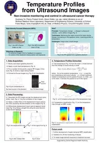
from Ultrasound Images Non-invasive monitoring and control in ultrasound cancer therapy Guoliang Ye, Penny Probert Smith, Alison Noble, {ye, pjp, noble} @robots.ox.ac.uk Wolfson Medical Vision Laboratory, Department of Engineering Science, University of Oxford Fares Mayia, fares.mayia@orh.nhs.uk, Dept. of Medical Physics, Churchill Hospital, Oxford. Temperature Profiles How? Principle: Temperature change change in ultrasound velocity echo shifts in image (Fig. 3) Techniques: Monitoring the region around the lesion during therapy, processing to find apparent strain, matching profiles to temperature Challenges: image noise, small change Fig 3: the RF signals from a gelatine phantom Objectives of Research: To enhance images (US) for feedback to surgeons To control of the treatment (head position and exposure) 1. Data Acquisition: 1.1 Build a test object (gelatine phantom) 1.2 Apply a cyclic heat (temperature) (Fig. 4) 1.3 For a number of time points, acquire RF images: A-line scan (Fig. 3) shows a region being heated 1.4 Convert to B-scan images (e.g. Fig. 5) for visualisation Fig 4:Cyclic temperature on the heat source in the phantom Fig 5: B-scan image 3. Temperature Profiles Extraction 3.1 Get temperature (Fig. 10) from the strain: a model derived from the change of sound velocity is used. where is the posterior temperature, , are the prior temperature and sound velocity, : a linear coefficient related to temperature and the speed of sound, C=1540, is the strain. n denotes the position on an A-line signal. 3.2 Temperature classification (Fig. 11) on the temperature map (through an MRF model) Fig 11: temperature maps before (left) and after (right) classification Heat source 2. Data Processing: 2.1 Resample the RF images and get the displacement (echo shifts) map (Fig. 6, 7) by the correlation of two images 2.2 Apply a median filter on the displacement map to reduce the noise caused by the decorrelation of the images (Fig. 8). 2.3 Differentiate displacement map to get an apparent strain map (Fig. 9) by fitting a straight line along the axial direction (Least Square Method) Fig 6: the displacement map Fig 7: A-line signal from fig. 6 Fig 8: after median filter Fig 9: strain Fig 10 : a 3-D shaded surface plot of the temperature map Future work 1. Further development of spatio-temporal MRF classification. 2. Validation for off-line monitoring of tissues. 3. To relate image-derived measures to treatment success. Supported by Oxford Regional Health Authority