Download
1 / 27
270 likes | 399 Views
Lecture 12 The Importance of Accurate Solar Wind Measurements. The Approach. Magnetospheric studies usually are based on a single solar wind monitor.

E N D
Lecture 12The Importance of Accurate Solar Wind Measurements
The Approach • Magnetospheric studies usually are based on a single solar wind monitor. • We propagate the solar wind from the observation point (usually the L1 point) to Earth by using the observed velocity and assuming that there are no changes along the way. • We assume that the solar wind is homogeneous across the width of the magnetosphere.
Characterizing the Solar Wind Parcels that Interact with the Earth • It has been recognized for a long time that simple propagation of the solar wind from a distant monitor to the Earth was flawed. • How well the IMF observed upstream actually represents the solar wind that interacts with the Earth depends on the separation of the spacecraft perpendicular to the Sun-Earth line. • Crooker et al., [1982] good correlation for d┴<50RE if the variance in the solar wind is large– good correlation for d┴<20RE if the variance is small. • Collier et al., [1998; 2000] have quantified the percentage of time two monitors observed good correlation as a function of d┴. A good correlation was >80%.
Characterizing the Solar Wind Parcels that Interact with the Earth 2 where L┴=41RE. • The Collier formula indicates at good correlations are found only 25% of the time for spacecraft with d┴~30RE. • Richardson and Paularena [2001] found evidence for scale lengths perpendicular to the flow of 45RE the IMF, 70RE for the speed and 100RE for the density. • The radial scale length is 400RE. • The entire potential difference across the magnetosphere only requires 3-4RE [Burke et al., 1999]. • Since this is much smaller than the typical IMF scale length perhaps transverse variations in the solar wind are not too important for the magnetosphere.
Propagating the Solar Wind • Weimer et al., in a series of papers suggested that by calculating a phase front the estimate of the time to propagate from L1 to the Earth could be improved. • Two methods have been used over the past couple of years. • MVAB-0 – calculated the minimum variance direction constrained such that the average field along the minimum variance direction is zero. (Haaland et al., [2006]; and an equivalent approach by Bargatze et al., [2005]) • For a set of magnetic field meaurements: The eigenvectors of give the maximum, intermediate and minimum variation of the field components. • Cross product – take the vector cross product of average magnetic field vectors upstream and downstream of the discontinuity.
Calculating the Phase Fronts • Red give phase fronts calculate from MVAB-0 and blue uses the cross product method. (Weimer and King, 2008)
Pick the Best Method at Each Time • Where there is disagreement use the method closest to the trend.
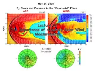
Predicted Lags • Top – convection delay; bottom – delay using combined method. • Separation (227.3RE, 5.4RE, 14.4RE)
Spacecraft Orbits on May 24, 2000 (Ashour-Abdalla, 2008) DAWN DUSK • Four solar wind monitors were available throughout most of the interval. • ACE was at the L1 point at x=220RE, Y=25 RE and Z=-20RE • Wind was moving toward the Earth about 60RE upstream, at noon and in the equator. • IMP-8 was duskward of noon, about 30RE upstream and 20RE below the ecliptic. • Geotail was at noon and crossed the bow shock during the interval.
ACE Solar Wind Observations During the May 23-24, 2000 Magnetic Storm • A magnetic cloud passed the Earth on May 23-24, 2000. • The solar wind dynamic pressure exceeded 30nPa. • A moderate storm (Dst~-150nT) resulted. • We have divided our analysis into two intervals • 2200UT May 23 to 0600UT May 24. The main body of the cloud passed the Earth. • 0900UT to 1500UT May 24. The magnetosphere was engulfed in the wake of the cloud.
Solar Wind and IMF Observations from Wind, ACE and IMP-8 – First Interval, May 23 and 24, 2000
Solar Wind and IMF Observations from Wind, ACE and IMP-8 – Second Interval, May 24, 2000
A Digression on Correlation • The cross correlation of two time series a and b is defined by where k is the lag, N and M are the lengths of the time series. • The sum is over all N+M+1 possible products. • An autocorrelation is a cross correlation of a time sequence with itself. • The correlation coefficient is equal to the cross correlation normalized to give one when the two time series are identical (perfectly correlated). • ψk is 1 for perfect correlation and -1 for anticorrelation.
Cross Correlation Between ACE and Wind BZ • The ACE data have been shifted 31:32 minutes with respect to Wind. • The cross correlation is >.95 with <2min additional shift. • The small shift may be do to changes in solar wind velocity between the two spacecraft.
Cross Correlation Between ACE and Wind BZ Second Interval. • The cross correlation is <0.7 with no dominant peak. • Delays of 2 hours are as good as zero. • The differences are not in the propagation scheme.
Peak Cross Correlations in IMF Bz Between ACE, Wind and IMP-8 Observations • Peak cross correlations were calculated over 2 hour running intervals. • Cross correlations are larger during the first interval. • Cross correlations in first interval improved with averaged data. • Best cross correlations occur between IMP-8 and Wind • Cross correlations during the second interval are not improved by averaging. • Similar results were found with up to 30 minute averages. No Smoothing Ten Minute Running Averages
Peak Cross-correlations in Dynamic Pressure Between IMP-8, ACE, and Wind Observations • Low cross-correlations for all three combinations when the data with no smoothing are used. • In general the IMP-8 and Wind observations agree best. • Averaging improves the cross-correlations for the first interval (especially IMP-8 and Wind early during the large pressure increase). • The cross-correlations during the pressure increase in the second interval become worse. No Smoothing Ten Minute Running Average
Organizing the Results • The magnetosphere is a complex time dependent three-dimensional structure. • The “equator” is a twisted surface located above the GSE equator on the dawn side and below it on the dusk side. • The cross section varies with X and time. • It’s cross section depends on the history of the solar wind and the resulting dynamics. • Needed to develop a way to organize the results.
Displaying the Results • The plasma sheet is the maximum pressure surface. • The color spectrogram gives the north-south component of B. • The white arrows show the flow. • The contours give the thermal pressure.