News from the Bioconductor project Genetic interactions Multiple testing and independent filtering

1. News from the Bioconductor projectGenetic interactionsMultiple testing and independent filtering Praha, 26 Aug 2009 Wolfgang Huber EMBL

2. An international open sourceand open development software project for the analysis of genomic data Use the statistical environment and language R as the integrating middleware Design principles: rapid development, code re-use Six-monthly release cycle; release 1.0 in March 2003 (15 packages), …, release 2.4 in April 2009 (320 packages)‏

3. Goals • Provide access to powerful statistical and graphical methods for the analysis of genomic data • Facilitate the integration of biological metadata (e.g. EntrezGene, BioMarts, PubMed) in the analysis of experimental data • Promote the development of accessible, extensible, transparent and well-documented software • Promote reproducible research • Provide training in computational and statistical methods

4. Good scientific software is like a good scientific publication Reproducible Subject to peer-review Easy to access and use by others Builds on the work of others Others can build their work on top of it

5. 320 packages in release 2.4, April 09 (60 more than last year) • Packages represent the work of 210 different researchers • 76 Pubmed citations between January 2008 and May 2009 • Original Bioconductor paper has over 1450 citations • Website sees over 14,000 unique visitors per month • Biobase package was downloaded to 34,354 unique IP addresses in the last year • Mailing lists have nearly 3000 subscribers, ~450 posts per month • New list dedicated to short read sequence analysis • In 2008, 8 Bioconductor courses; all at or near capacity • 80 participants attended annual conference, BioC2009

6. Bioconductor Short Course: Brixen, South Tyrol annually in June since 2004, 1 week Bioconductor Conference: Seattle, WA, annually late July Developer Meeting: Dec 09 in Manchester UK Many further short courses & developer meetings: see www.bioconductor.org!

7. How to get started Go to www.bioconductor.org and follow installation instructions (Linux, Windows, Mac) Read the book Subscribe to the mailing list Answer questions Contribute your own package!

8. Recent developments: next-generation sequencing ShortRead package data management (raw reads, alignments to reference genome e.g. from Bowtie, SAM-tools) data quality assessment Biostrings efficient string and alignment algorithms let you experiment with your own ideas IRanges efficient working with interval-type data and annotation along chromosomes

9. Recent developments: next-generation sequencing BSgenome data packages genome sequences of many model organisms rtracklayer view your data with a genome browser HilbertVis 2D embedding (Hilbert-curve) plots of along-genome data chipseq identify enriched regions GenomeGraphs make your own, custom along-chromosome plots

10. Hilbert curve, iteration 4

11. Hilbert plots of chromosome 10 H3K4me1 H3K4me3

12. 3-colour Hilbert plot red: H3K4me1 green: H3K4me3 blue: exons HilbertVis package

13. Recent developments: preprocessing and data quality report generation ShortRead short read data arrayQualityMetrics expression microarrays flowQ Flow cytometry cellHTS2

14. Recent developments: high content / high throughput assays cellHTS2 RNAi and compound screening with cell-based assays flow*gating and normalisation for flow cytometry data EBImage segmentation of 2D images of cells, feature extractionimageHTS (coming soon) complete data analysis workflow for large-scale microscopy imaging based screens

16. Complex traits Do not follow Mendelian inheritance and result from multiple alleles Responsible alleles contribute different amounts to phenotype Alleles may be present in only a fraction of all individuals with the phenotype

17. The genetic basis of complex traits Currently ~400 variants that contribute to common traits and diseases are known Even when dozens of genes have been linked to a trait, both the individual and the cumulative effects are disappointingly small (<5%) Limitations to current genome-wide association studies: Common SNPs miss rare variants with potentially huge effects Common variants with low penetrance also missed Many structural variants go undetected because they do not alter SNP sequences Epistasis, where the effect of one variant cannot be found without knowing the other, confounds identification Picture emerges that complex traits are conditioned by many common variants with different effect sizes and frequencies

18. Genetic architecture of complex traits: Largephenotypic effects and pervasive epistasisSinger et al. Science 2004, Shao et al. PNAS 2008 (J. Nadeau lab) C57BL/6J A/J differ for many physiological, morphological, behavioral, immunological, and oncological traits, including models of birth defects and adult diseases in humans

19. CSS Panels Chromosome substitution strains (CSS) panel: Strain CSS-i carries both copies of chromosome i from donor strain, but all other chromosomes from the host strain are intact and homozygous. Creation of C57BL/6J - A/J panel required more than 17,000 mice and took about 7 years. (With up-to-date selective breeding and genotyping, now estimated to be feasible in 4 years.) host donor IIIIIIIIII IIIIIIIIII

20. Phenotyping of 90 different complex traits 41 traits significantly different between parentals Per trait, there are on average 8 significant CSSs Average phenotypic effect per chromosome: 76% of the total

21. Effects are often not additive

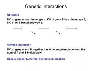
22. Interactions Additive model for quantitative trait Y General model with interactions Xi : genotype at locus i bij : interaction effect of loci i, j bi : main effect of locus i

23. viability A B X viability A*B* wt A* B* B A A*B* wt A* B A Types of interactions positive (synergistic) interaction negative (buffering)‏ interaction viability B* negative (suppressing) interaction A*B* wt A* B*

24. Combinatorial RNAi to systematically map all pairwise interactionsT. Horn, T. Sandmann, M. Boutros (DKFZ); E. Axelsson (EBI) X dsRNAs 384-well plate 384-well plate >3500 PP x PP (quadruplicates) PP x positive controls PP x negative controls PP alone Arrays of RNAi reagents

25. Estimating genetic interactions Data: log (cell viability) viability hits Pij = Wi + Wj + Wij obtain estimates for Wi, Wj, Wij by minimizing single effects synergistic interactions antagonistic interactions interactions

26. cluster of lipid phosphatases (CG11437, CG11438, wun) interact with JNK signaling Related phosphatases share interaction profiles Wij synergistic antagonistic

27. Example: rescue from DIAP1 DIAP, Drosophila Inhibitor of Apoptosis co-depletion with P71 shows rescue phenotype reproducible in different cell lines S2 A*B* wt A* B* negative (suppressing) interaction

28. Protein networks based on synthetic genetic interactions • Limited number of PP with many interactions, e.g. • puc • PP1- a96 • Expansion to larger network sizes, more complex phenotypes • Application to RNAi-drug interactions

29. Next Steps Microscopy Imaging - multivariate phenotypes: not just overall cell number, but morphological parameters of each invidual cell (cytokinesis defects, differentiation, apoptosis) Scale up to larger matrices (1000 x 1000 is feasible) Not just overall knock-down, but allele-specific perturbations in diploid backgrounds Aim: multivariate phenotype-genotype models with predictive value for phenotype engineering and rational drug therapy

30. Independent filters andmultiple testing Wolfgang Huber (EMBL/EBI) Richard Bourgon (EMBL/EBI) Robert Gentleman (FHCRC)

31. Multiple testing • Many data analysis approaches in genomics rely on item-by-item (i.e. multiple) testing: • Microarray expression profiles of “normal” vs “perturbed” samples: gene-by-gene • ChIP-chip: locus-by-locus • RNAi and chemical compound screens • Genome-wide association studies: marker-by-marker • QTL analysis: marker-by-marker and trait-by-trait

32. Multiple testing • Classical hypothesis test: • null hypothesis H0, alternative H1 • test statistic X  t(X)  • a = P( t(X) Grej | H0) type I error (false positive) • b = P( t(X) Grej | H1) type II error (false negative) • When n tests are performed, what is the extent of type I errors, and how can it be controlled? • E.g.: 20,000 tests at a=0.05, all with H0 true: expect 1,000 false positives

33. Experiment-wide type I error rates Family-wise error rate: P(V > 0), the probability of one or more false positives. For large m0, this is difficult to keep small. False discovery rate: E[ V / max{R,1} ], the expected fraction of false positives among all discoveries. Slide34

34. p-values: a mixture null alternative Slide35

35. Example: differential expression testing Acute lymphocytic leukemia (ALL) data, Chiaretti et al., Clinical Cancer Research 11:7209, 2005 Immunophenotypic analysis of cell surface markers identified T-cell derivation in 33, B-cell derivation in 95 samples Affymetrix HG-U95Av2 3’ transcript detection arrays with ~13,000 probe sets Chiaretti et al. selected probesets with “sufficient levels of expression and variation across groups” and among these identified 792 differentially expressed genes. Clustered expression data for all 128 subjects, and a subset of 475 genes showing evidence of differential expression between groups

36. Independent filtering From the set of 13,000 probesets, first filter out those that seem to report negligible signal (say, 40%), then formally test for differential expression on the rest. Conditions under which we expect negligible signal : Target gene is absent in both samples. (Probes will still report noise and cross-hybridization.) Probe set fails to detect the target. Literature: von Heydebreck et al. (2004)McClintick and Edenberg (BMC Bioinf. 2006) and references thereinHackstadt and Hess (BMC Bioinf. 2009) Many others. Slide37

37. Increased detection rates Stage 1 filter: compute variance, across samples, for each probeset, and remove the fraction θ that are smallest Stage 2: standard two-sample t-test ALL data

38. Increased detection rate implies increased power only if we are still controlling type I errors at the nominal level. Increased power? • Concerns: • Have we thrown away good genes? • Use a data-driven criterion in stage 1, but do type I error consideration only on number of genes in stage 2 • Informal justification: • Filter does not use covariate information (T-/B-cell type) ALL data Slide39

39. Non-specific filtering? • An informal explanation has been that the filtering “does not use any information from the class labels”. However, this is not enough, as these examples show: • Unsupervised clustering of the samples into two groups, filter by t-statistic for these groups, then test by t-statistic for actual groups. Asymptotically, and for certain data, • stage 1 statistic  stage 2 statistic • 2. Certain null distributions of the data that are not rotation symmetric (but iid).Then, • Lt ≠ Lt | s

40. Result: independence of stage 1 and stage 2 statistics under the null hypothesis For genes for which the null hypothesis is true (X1 ,..., Xn exchangeable), f and g are statistically independent in both of the following cases: • Normally distributed data: f (stage 1): overall variance (or mean) g (stage 2): the standard two-sample t-statistic, or any test statistic which is scale and location invariant. • Non-parametrically: f: any function that does not depend on the order of the arguments. E.g. overall variance, IQR. g: the Wilcoxon rank sum test statistic. Both can be extended to the multi-class context: ANOVA and Kruskal-Wallis. Slide41

41. Derivation Non-parametric case: Straightforward decomposition of the joint probability into product of probabilities using the assumptions. Normal case: Use the spherical symmetry of the joint distribution, p-dimensional N(0, 1s2), and of the overall variance; and the scale and location invariance of t. This case is also implied by Basu's theorem (V complete sufficient for family of probability measures P, T ancillary  T, V independent)

42. Type I error control requires • 1. Correct specification of the the marginal distribution of the test statistic for the true nulls. • 2. A dependence structure which is appropriate for the multiple testing method being used.  more subtle

43. How multiple testing procedures deal with dependence • 1. Methods that work on the p-values only and allow general dependence structure: Bonferroni, Bonferroni-Holm (FWER), Benjamini-Yekutieli (FDR) • 2. Those that work on the data matrix itself, and use permutations to estimate null distributions of relevant quantities (using the empirical correlation structure): Westfall-Young (FWER) • 3. Those that work on the p-values only, and require dependence-related assumptions: Benjamini-Hochberg (FDR), q-value (FDR)

44. Now we are confident about type I error, but does it do any good? (power)

45. q

46. Diagnostics odds ratio = 4.4 abs. value of t-statistic (stage 2) ALL data overall standard deviation (stage 1)

47. Results summary • There are cases in which "filtering" leads to incorrect type-I error control. • In other cases, the stage-one (filter) and stage-two (differential expression) statistics are marginally independent: • (Normal distributed data): overall variance or mean, followed by t-test • Any permutation invariant statistic, followed by Wilcoxon rank sum test • Marginal independence is sufficient to maintain control of FWER at nominal level. • Marginal independence does not preclude changes to correlation structure in filtered data: control of FDR not guaranteed; this is not likely a problem in practice.

48. Conclusion • Correct use of this two-stage approach can substantially increase power at same type I error. • Why does it work? • The filtering step is an (informal) way to bring in additional knowledge about the data (a „model refinement“)

49. EMBL Premier lab for biological research in Europe, with five sites, in Heidelberg, Cambridge (UK), Grenoble (F), Rome and Hamburg. Cell biology, Biophysics, Developmental Biology, Structural Biology, Genome Biology, Computational Biology EMBL

50. Simon Anders Elin Axelsson Ligia Bras Richard Bourgon Bernd Fischer Audrey Kauffmann Gregoire Pau Thank you Robert Gentleman, F. Hahne, M. Morgan (FHCRC) Lars Steinmetz, J. Gagneur, Z. Xu, W. Wei (EMBL) Michael Boutros, F. Fuchs, D. Ingelfinger, T. Horn, T. Sandmann (DKFZ) Steffen Durinck (Illumina) All contributors to the R and Bioconductor projects