Download
1 / 9
170 likes | 859 Views
Spring 2008. Discrete-Time Convolution. Linear Systems and Signals Lecture 8. Linear Time-Invariant System. Any linear time-invariant system (LTI) system, continuous-time or discrete-time, can be uniquely characterized by its Impulse response : response of system to an impulse

E N D
Spring 2008 Discrete-Time Convolution Linear Systems and SignalsLecture 8
Linear Time-Invariant System • Any linear time-invariant system (LTI) system, continuous-time or discrete-time, can be uniquely characterized by its • Impulse response: response of system to an impulse • Frequency response: response of system to a complex exponential e j 2 p f for all possible frequencies f • Transfer function: Laplace transform of impulse response • Given one of the three, we can find other two provided that they exist May or may not exist May or may not exist
passband Example Frequency Response • System response to complex exponential e jw for all possible frequencies wwherew = 2 p f • Passes low frequencies, a.k.a. lowpass filter |H(w)| H(w) stopband stopband w w -ws -wp wp ws Phase Response Magnitude Response
d[n] n Kronecker Impulse (Function) • Let d[n] be a discrete-time impulse function, a.k.a. the Kronecker delta function: • Impulse response h[n]: response of a discrete-time LTI system to a discrete impulse function 1
h[n] Averaging filter impulse response n 0 1 2 3 Discrete-time Convolution • Output y[n] for inputx[n] • Any signal can be decomposedinto sum of discrete impulses • Apply linear properties • Apply shift-invariance • Apply change of variables y[n] = h[0] x[n] + h[1] x[n-1] = ( x[n] + x[n-1] ) / 2
Comparison to Continuous Time • Continuous-time convolution of x(t) and h(t) • For each value of t, we compute a different (possibly) infinite integral. • Discrete-time definition is the continuous-time definition with integral replaced by summation • LTI system • If we know impulse response and input, we can determine the output • Impulse response uniquely characterizes it
Fundamental Theorem • The Fundamental Theorem of Linear Systems • If one inputs a complex sinusoid into an LTI system, then the output will be a complex sinusoid of the same frequency that has been scaled by the frequency response of the LTI system at that frequency • Scaling may attenuate the signal and shift it in phase • Example in continuous time: see handout G • Example in discrete time. Let x[n] = e j W n,H(W) is the discrete-time Fourier transform of h[n] and is also called the frequency response
Convolution Demos • Johns Hopkins University Demonstrations http://www.jhu.edu/~signals Convolution applet to animate convolution of simple signals and hand-sketched signals Convolve two rectangular pulses of same width gives a triangle
h[n] First-order difference impulse response n • Five-tap discrete-time (scaled) averaging FIR filter with input x[n] and output y[n] Lowpass filter (smooth/blur input signal) Impulse response is {1, 1, 1, 1, 1} • First-order difference FIR filter Highpass filter (sharpensinput signal) Impulse response is {1, -1}