Download
1 / 25
250 likes | 333 Views
Explore binomial distributions, probabilities, and settings for counts of successes in fixed observations, with examples and cautionary notes. Learn how to use binomial probability tables to calculate outcomes.

E N D
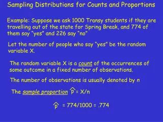
Sampling Distributions for Counts and Proportions The sample proportion = X/n p p Example: Suppose we ask 1000 Transy students if they are travelling out of the state for Spring Break, and 774 of them say “yes” and 226 say “no” Let the number of people who say “yes” be the random variable X. The random variable X is a count of the occurrences of some outcome in a fixed number of observations. The number of observations is usually denoted by n = 774/1000 = .774
The Binomial Setting 1) There are a fixed number n of observations 2) The n observations are independent 3) Each observation falls into just one of two categories, which, for convenience, we call “success” and “failure”. 4) The probability of a success, call it p, is the same for each observation
The Binomial Setting Example: Toss a fair coin 10 times, and count the amount of heads which will appear. The random variable, X, is the number of heads that appear. The probability of a success is p = 0.5 This experiment follows the four requirements for the Binomial Setting, so this is a Binomial Distribution.
Binomial Distributions The distribution of the count X of successes in the binomial setting is called the binomial distribution with parameters n and p. The parameter n is the number of observations The parameter p is is the probability of a success on any one observation. The possible values of X are the whole numbers from 0 to n. We say that X is B(n,p)
Binomial Distributions In the previous example, our distribution is B(10, 0.5) New example: Draw a card from a deck and determine if it is a spade or not. Return the card to the deck, shuffle, and repeat fourteen more times. Are we in the binomial setting? This is a B(15, 0.25) Q: Is there ever a situation where we are “close enough” to use the binomial distribution?
Binomial Distributions Example: Imagine we have a big ol’ bunch of transistors, say roughly 10,000. We will say that 1000 of them are bad. Pull an SRS of size 10 without replacement. Let X be the amount of transistors which are bad in the SRS. Q: Is this the binomial setting? A: No. The first transistor has a 1000/10,000 = 0.1 chance of being bad. What about the second? The second has either a 1000/9,999 = 0.10001 or 999/9,999 chance = 0.09991 chance of being bad We can consider this a B(10,0.1)
Sampling Distribution of a Count When the population is much larger than the sample, the count X of successes in an SRS of size n has approximately the B(n,p) distribution. Note: We will use the binomial sampling distribution for counts when the population is at least 10 times as large as the sample. Q: How can we find these binomial probabilities? A: Tables
Binomial Probability Tables (Table C, page T-7 to T-10) Consider the previous transistor problem using the B(10,.1) distribution. Q: What is the probability that we will pull an SRS from this distribution with exactly one bad transistor? A: P(X = 1) = 0.3874
Binomial Probability Tables (Table C, page T-7 to T-10) Consider the previous transistor problem using the B(10,.1) distribution. Q: What is the probability that we will pull an SRS from this distribution with at most one bad transistor? A: P(X 1) = P(X=0) + P(X=1) = 0.3487 + 0.3874 = 0.7361
Binomial Probability Tables (Table C, page T-7 to T-10) Consider the previous transistor problem using the B(10,.1) distribution. Q: What is the probability that we will pull an SRS from this distribution with an even number of bad transistors? A: P(X=2 or X=4 or X=6 or X=8 or X=10) = P(X=2) + P(X=4) + P(X+6) + P(X=8) +P(X= 10) = .3487 + .1937 + .0112 + .0001 + .0000 = .5537
Cautions about the Binomial Tables Do you notice anything about Table C? The values of p are all 0.5 or smaller. You need to adjust your count so you are using probabilities that are at most 0.5 Example: Suppose I shoot free throws at a 92% rate of success. What is the probability I make 10 out of twelve? This is a B(12, 0.92) distribution.
Cautions about the Binomial Tables Example: Suppose I shoot free throws at a 92% rate of success. What is the probability I make ten out of twelve? This is a B(12, 0.92) distribution. We can re-word this as follows: Example: Suppose I shoot free throws at an 8% rate of failure. What is the probability that I will miss two out of twelve? This is a B(12, 0.08) distribution. A: P(X=2) = .1835
Binomial Mean and Standard Deviation X = np (1-p) Q: If a count X is B(n,p), what are the mean X and the standard deviation X ? A: If a count X has the B(n,p) distribution, then : X = np
Binomial Mean and Standard Deviation X = np (1-p) = (12)(0.08)(0.92) = 0.9398 = 0.8832 Example: Refer back to the free throw example. The rate of misses was a B(12, 0.08) X = np = (12)(0.08) = 0.96
Count of successes in sample = Size of sample p X = n Sample Proportions In statistical sampling, we often want to estimate the proportion p of “successes” in a population. Our estimator is the sample proportion of successes :
Deep Thoughts • The proportion does not have a binomial • distribution, however, we can restate the • proportion as a count and proceed from there p Notice the difference between count and proportion : • The count is an integer between 0 and n • The proportion is a number between 0 and 1 • In the binomial setting, the count has a binomial • distribution
= X/500 P( 0.80 ) p p Example: We are going to survey 500 Transy students to see if they like the new GE system. Suppose that 85% of all Transy students would answer “yes”. What is the probability that at least 80% would agree in the sample proportion ? The count X has binomial distribution : B(500, 0.85). The sample proportion is : We are trying to find : Notice that 80% of 500 is : (0.80)(500) = 400 This means we need to find : P( X 400) P( X 400) = P( X = 400) + P( X = 401) + … + P( X = 500)
Mean and Standard Deviation of a Sample Proportion Let be the sample proportion of successes in an SRS of size n drawn from a large population having population proportion p of successes. The mean and standard deviation of are the following : = p = p(1-p) p p p p n
Mean and Standard Deviation of a Sample Proportion (0.85)(0.15) = p = 500 = p(1-p) p p n Example: Refer back to the previous question about the new GE system. Q: What are the mean and standard deviation of the proportion of the survey respondents who like the new GE system? A: = 0.85 = 0.0159687
Deeper Thoughts • Recall that the sampling distribution of a sample proportion • is close to normal. (See section 3.4, p. 270) • Both the count X and the sample proportion are • approximately normal when we have a large sample. • We can use the normal curve to solve some difficult • binomial distribution problems !
Normal Approximations for Counts and Proportions • Let X be the count of successes in the sample, and • = X / n be the sample proportion of successes. • X is approximately N( np, np(1-p) ) ( p, ) p(1-p) p p • is approximately N n • Draw an SRS of size n from a large population having • population proportion p of successes. • When n is large, the sampling distributions of these • statistics are approximately normal. Note: Use this when np 10 and n(1-p) 10
Normal Approximations for Counts and Proportions = X/500 P( 0.80 ) p p Example: We are going to survey 500 Transy students to see if they like the new GE system. Suppose that 85% of all Transy students would answer “yes”. What is the probability that at least 80% would agree in the sample proportion ? The count X has binomial distribution : B(500, 0.85). The sample proportion is : We are trying to find : Notice that 80% of 500 is : (0.80)(500) = 400 This means we need to find : P( X 400) P( X 400) = P( X = 400) + P( X = 401) + … + P( X = 500)
Normal Approximations for Counts and Proportions • X is approximately N( (500)(0.85), (500)(0.85)(0.15) ) • X is approximately N( np, np(1-p) ) 400 - 425 8 In this example : • X is approximately N( 425, 8 ) P( X 400) We are trying to find : Z = = -3.13 .9991 = 99.91%
Normal Approximations for Counts and Proportions • is approximately N(0.85, 0.0159687) 0.80 - 0.85 0.0159687 ( p, ) P( 0.80 ) p(1-p) p p p • is approximately N n In this example : We are trying to find : Z = = -3.13 .9991 = 99.91%
Homework 2, 4, 6, 8, 12, 14, 22, 24