Sensitivity of a Simplified Tropical Cyclone Intensity Model to the Thermodynamic Environment

1. Sensitivity of a Simplified Tropical Cyclone Intensity Model to the Thermodynamic Environment Mark DeMaria, RAMM Branch NOAA/NESDIS/StAR, Fort Collins, CO IUGG Conference July 2007 Perugia, Italy

2. Outline • Intensity Forecast Trends • Hierarchy of TC forecast models • A new statistical-dynamical intensity model • Estimating intensity upper bound • Estimating TC growth rates • Thermodynamic sensitivity • Forecast applications

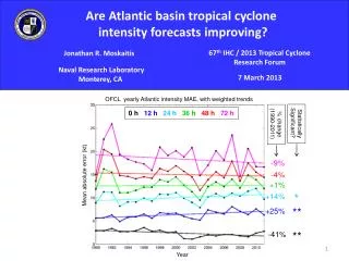
3. Mean Absolute Error of NHC Official Atlantic Track and Intensity Errors1985-2006 Track Intensity 3.5% Per Year 0.8% Per Year

4. Tropical Cyclone Intensity Forecasting • Less skillful than track forecasts • Numerical forecasts often inaccurate • Greater reliance on extrapolation, empirical and statistical forecast methods • Intensity change sensitive to wide range of physical processes • eyewall and other convection • boundary layer and air-sea interaction • microphysical processes • synoptic scale interaction • land interaction

5. NHC Tropical Cyclone Intensity Forecast Models • Operational Models • SHIFOR: Very simple regression model with climatology and persistence input • Used as skill baseline • SHIPS: Statistical-dynamical linear regression model with atmospheric, oceanic, climatological and persistence predictors • GFS: NCEP global forecasting system • GFDL: NCEP version of GFDL coupled ocean-atmosphere model • H-WRF: NCEP Hurricane WRF coupled ocean-atmosphere model • Operational for 2007 • Experimental Models • CHIPS: - K. Emanuel simplified 2-D coupled ocean-atmosphere model • FSU super-ensemble: Provides optimal combinations of other models

6. Skill No Skill Skill of NHC Intensity Forecast Models

7. New Statistical-Dynamical Intensity Prediction Model • More complex than linear regression (SHIPS) • Less complex than deterministic prediction systems • Use physical reasoning when possible • Incorporate upper bound estimate • Growth rate modified by dynamical and thermodynamic effects

8. A Short Biology Lesson:Population Growth dP/dt = rP - P2 rP = reproduction term, P2 = Mortality term P = population r,  = species parameters Let = r/K, K=“Carrying capacity” related to food supply for given species dP/dt = rP( K-P)/K If P << K, dP/dt = rP, P(t) = Poert If dP/dt = 0 (steady state), P(t) = K

9. Two Strategies for Species Survival • r-selected (P << K) • Large reproductive rates • Most offspring don’t survive to adults • Adults don’t care for young • Population usually well below carrying capacity • e.g., Insects, amphibians, crustaceans • K-selected (P~K) • Small reproductive rates • Adults care for young • Populations close to carrying capacity • Very sensitive to environment changes, species loss • e.g., Most large mammals

10. Application to TC Intensity PredictionLogistic Growth Equation (LGE) Model dV/dt = V - (V/Vmpi)nV (A) (B) Term A: Growth term, related to shear, structure, etc Term B: Upper limit on growth as storm approaches its maximum potential intensity (Vmpi) Assume: , n are constants for all storms Vmpican be calculated given SST, Tupper, etc  is storm, time dependent Fit above model to SHIPS data set: 1) Determine universal values of , n n=2.5, -1=24 hr 2) Estimate (t) and Vmpi(t) for prediction model

11. Analytic LGE Solutions for Constant Vmpi and for n=3 Vs = Steady State V = Vmpi(/)1/3 V/Vs = (Vo/Vs)et/[1 + (e3t-1)(Vo/Vs)3]1/3   0   0

12. Estimation of Vmpi • Miller (1958) • Min pressure estimated by estimate from eye subsidence and environmental sounding • Holland (1997) • Refinement of Miller method • Emanuel (1987, 1995, 1998) • Based on Carnot heat engine • Vmpi = f(SST, Toutflow, RH sfc) • DeMaria and Kaplan (1994) • Assume Toutflow = f1(SST) and RHsfc = f2(SST) • Emanuel formula reduces to Vmpi = F(SST) • Determine F(SST) empirically from observations

14. Observed  Distribution(7580 Atlantic cases 1982-2005) -1 = 200 hr 67 hr 40 hr 29 hr 22 hr 18 hr  = (1/V)dV/dt + (V/Vmpi)n

15. (t) for Hurricane Frances 2004 =0.02  -1 = 50 hr =0.03  -1 = 33 hr

16. Hurricane Frances (2004) LGE Model Solution with two  values -1 = 44hr 082500 to 090118 -1 = 82hr 090200 to 090500

17. Estimation of  • Assume  depends on storm environment • Vertical shear of horizontal wind (S) • S is modified by latitude in support of observations • S = S’[1-0.8sin()] • S’ = 200-850 hPa vertical wind shear •  = latitude • Potential to support convection (C) • Need a measure of tropical convective potential

18. Tropical Convection • “Hot Towers”: un-dilute ascent from surface to the tropopause • CAPE or Lifted Index could be used • Hot towers not supported by most observations • Expected updrafts way too large • Hot tower modifications • Entrainment • Effect of liquid water weight on buoyancy • Non-hydrostatic pressure gradients

19. Mean Atlantic Hurricane Season Sounding* “Hot Tower” CAPE = 3970 J/kg *From J. Dunion (2007) for non-Sarahan Air Layer composite

20. Entraining Parcel Model • Lagrangian parcel model with Ooyama (1990) thermodynamic formulation • Prognostic variables • 1) Vertical velocity, 2) entropy mixing ratio, 3) total condensate mixing ratio, 4) total parcel mass • Single condensate: acts like liquid above 0oC and ice below 0oC • Entrainment included through specified entrainment rate • Buoyancy affected by condensate weight • Simple precipitation parameterization • Requires atmospheric T, RH sounding as input • Mean sounding from Atlantic hurricane season for testing • (J. Dunion 2007) • Soundings from NCEP GFS model for prediction

21. Parcel Vertical Velocities with Mean Hurricane Season Sounding

22. Model Sensitivity to Mid-level Moisture Saharan Air Layer (SAL) sounding from Dunion (2007) 30 to 40% RH reduction in 3 to 6 km layer

23. Estimation of  • Convective potential (C ) is the vertically averaged vertical velocity from the entraining parcel model • S is vertical shear modified by latitude •  = a0 + a1S + a2C + a3CS • Estimate a0,a1,a2,a3 byfit to observations of , S, C

24. (C,S)

25. Storm Behavior Depends on C,S Regime High • Rapid Intensification • Eyewall replacements • Storm growth through • symmetric processes • Transient behavior • Asymmetric convection • Storm growth through • asymmetric processes Convective Potential (C) • Dissipation • Extra-tropical transition • Growth through baroclinic • processes • Steady state storms • Annular hurricanes Low Low High Vertical Shear (S)

26. C-S Regime Examples • Katrina (AL 2005) C-S = High-Low • Daniel (EP 2006) C-S = Low-Low • Claudette (AL 2003) C-S = High-High

27. Hurricane Katrina 2005C-S = High-Low

28. Hurricane Daniel 2006C-S = Low-Low

29. Hurricane Claudette 2003C-S = High-High

30. LGE Forecast Applications • Use NHC operational forecast track • Ocean input from weekly Reynold’s SST • Atmosphere input from NCEP GFS model • MPI from DK empirical formula •  predicted statistically • LGE integrated numerically • Empirical decay for over-land track

31. LGE Model Forecast Tests2004-2006 Sample Percent Improvement over operational SHIPS model

32. Summary and Conclusions • TC intensity changes are more complex than track • Intensity forecasts are less skillful • Intensity changes can be approximated by a logistic growth equation (LGE) • The LGE model forecast skill is greater than the NHC operational linear regression model (SHIPS) • The TC growth rate depends on dynamic and thermodynamic properties of the environment • The convective response to thermodynamic changes is highly nonlinear • Storm behavior can partially be explained by a thermodynamic-dynamic phase space