Download

1 / 34
340 likes | 553 Views
Predictability of Tropical Cyclone Intensity Forecasting. Mark DeMaria NOAA/NESDIS/ StAR , Fort Collins, CO CoRP Science Symposium Fort Collins, CO August 2010. Outline. Overview of tropical cyclone intensity forecasting Charlie Neumann (1987) methodology

E N D
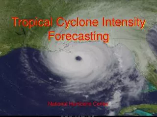
Predictability of Tropical Cyclone Intensity Forecasting Mark DeMaria NOAA/NESDIS/StAR, Fort Collins, CO CoRP Science Symposium Fort Collins, CO August 2010
Outline • Overview of tropical cyclone intensity forecasting • Charlie Neumann (1987) methodology • Use of statistical-dynamical models for predictability estimates • Predictability results
NHC 48 h Atlantic Track and Intensity Errors 1985-2009 Track 63% Improvement in 24 yr Intensity 9% Improvement in 24 yr HFIP Goals: 20% in 5 yr, 50% in 10 yr
Types of TC Intensity Forecast Models • Statistical Models: • SHIFOR, 1988(Statistical Hurricane Intensity FORecast) : Based solely on historical information - climatology and persistence (Analog to CLIPER) • Statistical/Dynamical Models: • SHIPS,1991(Statistical Hurricane Intensity Prediction Scheme): Based on climatology, persistence, and statistical relationships to current and forecast environmental conditions • LGEM, 2006 (Logistic Growth Equation Model): Variation on SHIPS, relaxes intensity to Maximum Potential Intensity (MPI) • Dynamical Models: • GFS, UKMET, NOGAPS, ECMWF • GFDL, 1995; HWRF 2007Solves the governing equations for the atmosphere (and ocean) • Ensemble, Consensus Models
Statistical / Dynamical Intensity ModelsSHIPS (Statistical Hurricane Intensity Prediction Scheme) • Multiple regression model • Predictors from climatology, persistence, atmosphere and ocean • Atmospheric predictors from GFS forecast fields • SST from Reynolds weekly fields along forecast track • Predictors from satellite data • Oceanic heat content from altimetry • GOES IR window channel brightness temperatures • Decay SHIPS • Climatological wind decay rate over land
The SHIPS Model Predictors* (+) SST POTENTIAL (VMAX-V): Difference between the maximum potential intensity (depends on SST) and the current intensity (-) VERTICAL (850-200 MB) WIND SHEAR: Current and forecast, impact modified by shear direction (-) VERTICAL WIND SHEAR ADJUSTMET: Accounts for shear between levels besides 850 and 200 hPa (+) PERSISTENCE: If TC has been strengthening, it will probably continue to strengthen, and vice versa (-) UPPER LEVEL (200 MB) TEMPERATURE: Warm upper-level temperatures inhibit convection (+) THETA-E EXCESS: Related to buoyancy (CAPE); more buoyancy is conducive to strengthening (+) 500-300 MB LAYER AVERAGE RELATIVE HUMIDITY: Dry air at mid levels inhibits strengthening *Red text indicates most important predictors
The SHIPS Model Predictors (Cont…) (+) 850 MB ENVIRONMENTAL RELATIVE VORTICITY: Vorticity averaged over large area (r <1000 km) – intensification favored when the storm is in environment of cyclonic low-level vorticity (+) GFS VORTEX TENDENCY: 850-hPa tangential wind (0-500 km radial average) – intensification favored when GFS spins up storm (-) ZONAL STORM MOTION: Intensification favored when TCs moving west (-) STEERING LAYER PRESSURE: intensification favored for storms moving more with the upper level flow – this predictor usually only comes into play when storms get sheared off and move with the flow at very low levels (in which case they are likely to weaken) (+) 200 MB DIVERGENCE: Divergence aloft enhances outflow and promotes strengthening (-) CLIMATOLOGY: Number of days from the climatological peak of the hurricane season
Satellite Predictors added to SHIPS in 2003 1. GOES cold IR pixel count 2. GOES IR Tb standard deviation 3. Oceanic heat content from satellite altimetry (TPC/UM algorithm) Cold IR, symmetric IR, high OHC favor intensification
Factors in the Decay-SHIPS ModelCenter over Water Normalized Regression Coefficients at 48 hr for 2010 Atlantic SHIPS Model
Regions with Most Favorable Shear Directions for Hurricane Ike(New SHIPS Model Predictor in 2009)
New LGEM and SHIPS Input for 2010 • Generalized Shear (GS) P2 GS = 4/(P2-P1)∫ [(u-ub)2 + (v-vb)2]1/2 dP P1 P1=1000 hPa, P2=100 hPa, ub,vb = mean u,v in layer • GS = 2-level shear for linear wind profiles
The Logistic Growth Equation Model (LGEM) • Applies simple differential equation to constrain the max winds between zero and the maximum potential intensity • Based on analogy with population growth modeling • Intensity growth rate predicted using SHIPS model predictors • More responsive than SHIPS to time changes of predictors such as vertical shear • More sensitive track errors • More difficult to include persistence
The Logistic Growth Equation Model • Uses analogy with population growth modeling • dV/dt = V - (V/Vmpi)nV • (A) (B) (C) • (A) = time change of maximum winds • Analogous to population change • (B) = growth rate term • analogous to reproduction rate • (C) = Limits max intensity to upper bound • Analogous to food supply limit (carrying capacity) • , n = empirical constants • Vmpi= maximum potential intensity (from empirical SST function) • = growth rate (estimated empirically from ocean, atmospheric predictors GFS,satellite data, etc)
Dynamical Intensity Models GFS: U.S. NWS Global Forecast System < relocates first-guess TC vortex UKMET: United Kingdom Met. Office global model < bogus (syn. data) NOGAPS: U.S. Navy Operational Global Atmospheric Prediction System global model < bogus (synthetic data) ECMWF: European Center for Medium-range Weather Forecasting global model (no bogus) GFDL: U.S. NWS Geophysical Fluid Dynamics Laboratory regional model <bogus (spin-up vortex) HWRF: NCEP Hurricane Weather Research and Forecast regional model (vortex relocation and adjustment)
Dynamical Intensity Model Limitations Sparse observations, especially in inner core Inadequate resolution, especially global models Data assimilation on storm scale Representation of physical processes PBL, microphysics, radiation Ocean interactions Predictability
The Geophysical Fluid Dynamics Laboratory (GFDL) Hurricane Model • Dynamical model capable of producing skillful intensity forecasts • Coupled with the Princeton Ocean Model (POM) (1/6° horizontal resolution with 23 vertical sigma levels) • Replaces the GFS vortex with one derived from an axisymmetric model vortex spun up and combined with asymmetries from a prior forecast • Sigma vertical coordinate system with 42 vertical levels • Limited-area domain (not global) with 2 grids nested within the parent grid • Outer grid spans 75°x75° at 1/2° resolution or approximately 30 km. • Middle grid spans 11°x11° at 1/6° resolution or approximately 15 km. • Inner grid spans 5°x5° at 1/12° resolution or approximately 9 km
The Hurricane Weather Research & Forecasting (HWRF) Prediction System • Next generation non-hydrostatic weather research and hurricane prediction system • Movable, 2- way nested grid (9km/27km; 42 vertical levels; ~75°x75°) • Coupled with Princeton Ocean Model • POM utilized for Atlantic systems, no ocean coupling in N Pacific systems • Vortex initialized through use of modified 6-h HWRF first guess • 3-D VAR data assimilation scheme • But with more advanced data assimilation for hurricane core • Use of airborne and land based Doppler radar data (run in parallel) • Became operational in 2007 • Under development since 2002 • Runs in parallel with the GFDL
*HWRF *GFDL *Configurations for 2010 season
Operational Intensity Model Verification (2007-2009 Atlantic)
Most Accurate Atlantic Early Intensity Models 1995-2009 (48 and 96 hr forecast) Year 1995 1996 1997 1998 1999 2000 2001 2002 2003 2004 2005 2006 2007 2008 2009 48-hr SHFRSHIP SHIPSHIPSHIP DSHP DSHPDSHPDSHPDSHPDSHPGFDLDSHP LGEM LGEM 96 hr SHIPGFSSHIPGFDLDSHPGFDLDSHPGFDLLGEM Statistical Statistical -Dynamical Global-Dynamical Regional-Dynamical
C. J. Neumann (1987)Prediction of Tropical Cyclone Motion: Some Practical Aspects • Most accurate track models were statistical-dynamical • Track error improvement ~0.5% per year • Error reductions leveling off • How much can track forecasts be improved? • Run NHC83 statistical-dynamical model with “perfect prog” input and compare runs with operational input • Showed 50% improvements were possible
Intensity Predictability Study • Use LGEM statistical-dynamical model • Run 4 versions • V1. NHC forecast tracks, GFS forecast fields • Operational input • V2. NHC forecast tracks, GFS analysis fields • V3. Best track positions, GFS forecast fields • V4. Best track positions, GFS analysis fields • V1. Provides current baseline • V4. Provides predictability limit • V2. Evaluates impact of large-scale improvement • V3. Evaluates impact of track improvement
Forecast Sample and Procedure • Use 2010 version of LGEM fitted to 1982-2009 developmental sample • Predictability analysis for Atlantic 2002-2009 sample • 135 tropical cyclones • 2402 forecasts to at least 12 h • 859 forecasts to 120 h • Compare LGEM with operational input to combinations of “perfect prog” track and GFS • Forecast verification using standard NHC rules
2002-2009 Intensity Errors OFCL = NHC operational forecasts Ver 1 = LGEM w\ oper input Ver 2 = LGEM w\ perfect GFS Ver 3 = LGEM w\ perfect tracks Ver 4 = LGEM w\ perfect tracks + GFS
LGEM Improvements over LGEM w\ Operational Input Perfect GFS Perfect track Perfect GFS & track
Illustration of Track Error1000 plausible Hurricane Ike tracks/intensities based on recent NHC forecast errors
Additional Improvements • TPW , Lightning density, µ-wave imagery input • Adjoint of LGEM to include storm intensity history up to forecast time • Consensus/ensembles • Dynamical model improvements under HFIP • Resolution, physics, assimilation
2-hourly Composite Lightning StrikesHurricane Ida 8 November 2009
Sample Text Output Lightning-Based Rapid Intensity Forecast Algorithm Hurricane Alex 30 June 2010 00 UTC
Conclusions • Current intensity forecast properties similar to those for track in 1980s • Neumann (1987) track predictability framework applied to intensity problem • LGEM statistical-dynamical model run with “perfect prog” input • 4%, 8%, 17%, 28%, 36% improvement at 1-5 day • About ½ might be realizable • Majority of intensity improvement from reducing track errors • Better dynamical models needed to achieve 10 year HFIP goal of 50% improvement