Finding Limits Graphically & Numerically
Finding Limits Graphically & Numerically. Section 1.2. After this lesson, you should be able to:. estimate a limit using a numerical or graphical approach determine the existence of a limit. Introduction to Limits. The function. is a rational function.

Finding Limits Graphically & Numerically
E N D
Presentation Transcript
Finding Limits Graphically & Numerically Section 1.2
After this lesson, you should be able to: • estimate a limit using a numerical or graphical approach • determine the existence of a limit
Introduction to Limits The function is a rational function. If I asked you the value of the function when x = 4, you would say ______ What about when x = 2? Well, if you look at the function and determine its domain, you’ll see that . Look at the table and you’ll notice ERROR in the y column for –2 and 2. On your calculator, hit then then . You’ll see that no y value corresponds to x = 2.
Continued… Since we know that x can’t be 2, or –2, let’s see what’s happening near 2 and -2… Let’s start with x = 2. We’ll need to know what is happening to the right and to the left of 2. The notation we use is: read as: “the limit of the function as x approaches 2”. In order for this limit to exist, the limit from the right of 2 and the limit from the left of 2 has to equal the same real number.
To take the right limit, we’ll use the notation, The + symbol to the right of the number refers to taking the limit from values larger than 2. To take the left limit, we’ll use the notation, The - symbol to the right of the number refers to taking the limit from values smaller than 2. Right and Left Limits
Right LimitNumerically The right limit: Look at the table of this function. You will probably want to go to TBLSET and change the TBL to be .1 and start the table at 1.7 or so. We can also set Indpnt to Ask and enter our own values close to 2. As x approaches 2 from the right (larger values than 2), what value is y approaching?
Left LimitNumerically The left limit: Again, look at the table. As x approaches 2 from the left (smaller values than 2), what value is y approaching?
The LimitNumerically Both the left and the right limits are the same real number, therefore the limit exists. We can then conclude, To find the limit graphically, trace the graph and see what happens to the function as x approaches 2 from both the right and the left. You can ZOOM IN to see x values very close to 2.
Take the limit from the right and from the left: Another Example: Finding Limit Numerically On your calculator, graph Where is f(x) undefined? Use the table on your calculator to estimate the limit as x approaches 0.
One more Example EXAMPLE: Find the numerically and verify graphically. Answer: *Use Radian mode.
Methods for finding limits Notation: roughly translates into: The value of f(x), as x approaches c from either side, becomes close to L. Limits can be estimated three ways: Numerically… looking at a table of values Graphically…. using a graph Analytically… using algebra OR calculus (covered next section)
Limits Graphically: Example 1 L1 There’s a break in the graph at x = c L2 c Although it is unclear what is happening at x= c since x cannot equal c, we can at least get closer and closer to c and get a better idea of what is happening near c. In order to do this we need to approach c from the right and from the left. Discontinuity at x = c Right Limit Left Limit
Note: The limit exists but L f(c) Limits Graphically: Example 2 L Hole at x = c c Right Limit Discontinuity at x = c Left Limit The existence or nonexistence of f(x) at x = c has no bearing on the existence of the limit of f(x) as x approaches c.
Limits Graphically: Example 3 No hole or break at x = c f(c) Right Limit c Left Limit Continuous Function In this case, the limit exists and the limit equals the value of f(c).
Limit Differs From the Right and Left- Case 1 To graph this piecewise function, this is the menu The limits from the right and the left do not equal the same number, therefore the limit ____________________________________.
Unbounded Behavior- Case 2 Since f(x) is not approaching a real number L as x approaches 0, the limit does not exist.
Oscillating Behavior- Case 3 Look at the graph of this function (in radian mode). Since f(x) is oscillates between –1 and 1 as x approaches 0, the limit does not exist.
A limit does not exist when: • f(x) approaches a different number from the right side of c than it approaches from the left side. (case 1 example) • f(x) increases or decreases without bound as x approaches c. (The functiongoes to +/- infinity as x c : case 2 example) • f(x) oscillates between two fixed values as x approaches c. (case 3 example)
Homework Section 1.2: page 54 #3, 7-15 odd, 19, 49, 53, 63, 65