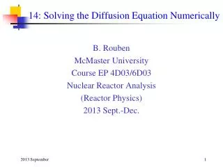
14: Solving the Diffusion Equation Numerically
14: Solving the Diffusion Equation Numerically. B. Rouben McMaster University Course EP 4D03/6D03 Nuclear Reactor Analysis (Reactor Physics) 2013 Sept.-Dec. Contents. We derive the finite-difference version of the 2-group diffusion equation and a method to solve it numerically.

14: Solving the Diffusion Equation Numerically
E N D
Presentation Transcript
14: Solving the Diffusion Equation Numerically B. Rouben McMaster University Course EP 4D03/6D03 Nuclear Reactor Analysis (Reactor Physics) 2013 Sept.-Dec.
Contents • We derive the finite-difference version of the 2-group diffusion equation and a method to solve it numerically.
Considering Real Reactors • Up to now we have considered very simple cases of homogeneous reactors. • Real life is more complicated, and real reactors have very complex, certainly not homogeneous, cores! • Therefore, analytic solutions to the flux shape in real reactors are not applicable. Instead, we must be prepared to solve the diffusion equation numerically. • Also, the 1-group treatment is not sufficiently accurate for real reactors. We must do diffusion calculations in at least 2 energy groups.
Diffusion Equation in 2 Energy Groups • Let’s start with the diffusion equation in 2 energy groups. • Let’s make a small simplifying concession: • We will assume that there is no upscattering from the thermal group to the fast group, only downscattering (moderation) from the fast group to the thermal group, and • We will assume that all fissions are thermal fissions, i.e., are induced by neutrons in the thermal group. • Also, we will work in 2 spatial dimensions instead of 3. • [These assumptions are not crucial, and do not simplify the method significantly, they just simplify the picture a bit.]
Notation • Let’s adopt the following notation: • Subscript 1 Fast group • Subscript 2 Thermal group • r position in 2 spatial dimensions (x, y) • D1(r), D2(r) Group diffusion coefficients • a1(r), a2(r) Group absorption cross sections • 12(r) Downscattering (moderation) cross section • f(r) Thermal fission cross section • keff Reactor multiplication constant
Diffusion Equation in 2 Energy Groups • The 2-group diffusion equation is then: • We have to get a solution which satisfies these equations at all points in the reactor. • Now we need to have a reactor model. See a model for a small “2-dimensional” reactor on the next slide. The reactor is modelled as square (rather than near-cylindrical) for simplicity.
2-D Reactor Model For Diffusion Calculation Legend Coloured Cells: Fuel of various burnups (channels refuelled at Various past times) Dimensions of Basic Cell=28.6 cm x 28.6 cm
Finite-Difference Method • We will apply the finite-difference method to solve for the flux at the midpoints of the cells defining the reactor model. Note that the assumption is made that the cells defined have homogeneous properties. That is, all cells of the same colour have the same properties; of course, outer-core, inner-core, and reflector properties are different! • The method should also produce the value of keff, which is not known a priori. • The finite-difference method gets its name from the fact that it approximates derivatives by finite-difference ratios. • The finite-difference method can be mesh-centred or edge-centred, depending on whether it solves for the flux at the centre or at the edge of the meshes. We will use the mesh-centred method.
Finite-Difference Method • The finite-difference method starts by integrating Eq. (1) over the volume of a cell, let’s label it with superscript C: • The integrals in Eq. (2) are of 2 kinds: those which involve the divergence operator, and those which don’t. • The integrals which do not involve the divergence are easy to deal with, taking advantage of the homogeneous properties. For example:
Finite-Difference Method (cont’d) • At this point we make the approximation that the volume integral of the flux is equal to the value at the centre of the cell times the volume of the cell, i.e.: • See a sketch on the next slide of cell C and its immediate neighbours on the left, right, top, and bottom (L, R, T, B respectively). Those are the neighbours we will need to calculate the leakage from cell C.
Integrals in the Divergence Operator • Let us now deal with the integrals in the divergence operator, i.e., integrals • These are the integrals which give the fast and thermal leakage out of cell C. Let’s work with the thermal group as an example.
Leakage Calculation in Finite Difference • Let’s do the surface integral by first doing the integral over one portion of the surface – say the interface between C and L. • In order to calculate the leakage in finite difference, we need to use the flux at the midpoint of each cell, and also the flux at the interface. • The basic figure we need for the calculation is shown in the next slide.
Leakage Calculation • To calculate the leakage, we first calculate the current (in the x direction) on each side of the interface CL, approximating the derivative of the flux by the first-order difference in fluxes between the midpoint of each cell and the (unknown) flux at the interface. We equate these two currents, since the current must be continuous at the interface: • We use this equation to solve for the interface flux. We get
Leakage Calculation (cont’d) • Substituting this back into the right-hand side of Eq. (7) to calculate J (we could equally have used the left-hand side): • To calculate the leakage from cell C across interface CL, we must take -Jx (since the outward normal to CL is towards -x) and multiply it by the “area” of the interface. This “area” is yC: the model is 2-dimensional, so we can take all cell “widths” in the 3rd dimension (z) to be unity. Therefore
Leakage Calculation (cont’d) • We could write Eq. (10) as • An exactly similar procedure can be used to derive the leakage across the other interfaces, so that we can write in the end
Leakage Calculation (cont’d) • If we put together everything we have derived, we can write the finite-difference form of Eq. (1) as: • Eq. (15) must be solved for every (cell) point (C) in the reactor model. This means that there is a system of [2 x the number of points in the model] coupled equations. • For the small 2-d model in slide 7, it’s a system of hundreds of coupled equations, and for a realistic reactor model it can be thousands or tens of thousands of coupled equations. • It is impossible to solve such large systems in one shot (i.e., “invert the matrix of the problem” in one shot). Thus, the solution must be by iteration.
Iterative Solution • The way that the iterative solution works is as follows: • Make an initial guess for the flux values (e.g., take the flux value to be the same at every point C). • Scan through the reactor points C one by one, solving the 2x2 system in Eq. (15) for the 2 flux values at C, using on the right-hand sides the current (latest) values of the flux at the neighbour points L, R, T, B, then proceeding to the next point C. This represents one “iteration”. • Repeat the scan of the reactor for another iteration (using as latest guess the flux values obtained at the previous iteration), then another, etc., until “convergence”. • Declare that convergence has been achieved when the ratio of the flux in the current iteration to that in the previous iteration, for every point in the reactor, is sufficiently close to 1 (i.e., the difference from 1 is smaller than a desired convergence criterion, e.g., 10-4 or10-5.)
Points at External Reactor Boundaries • Before we can actually embark upon the iterative solution, there is one thing that we must do: deal with the boundary points, which have no “neighbours”. • To deal with the boundaries, we make use of the extrapolation distance, dextr = 0.7104 tr (into a vacuum). • Consider a point C at the left edge of the reactor. It has no neighbour L, but we can pretend that it has a neighbour L where the flux is 0 at the extrapolation distance. For this “dummy neighbour cell”, the width will then be x = 2*dextr, so that the midpoint is at dextr. • See the sketch on the next slide.
Dummy Neighbour Cell Outside Reactor • We can pretend that the point C at the boundary has a neighbour cell outside the reactor, with difusion coefficient equal to the one in cell C, cell width 2*dextr, and flux = 0 at the midpoint. • i.e., for this dummy cell L:
Back to Iterative Solution • We can now perform the iterations, if we make and use a ring of “dummy” neighbours outside the external boundary, with properties as shown in the previous slide. • [Note: we do not solve for the flux in the dummy cells, we know that it is 0, we use them only as neighbours, as needed.] • One more thing: We need to determine keff as we iterate. We can start with a guess (e.g., keff = 1), and after each iteration j update keff by the ratio of total flux in the reactor to that in the previous iteration, as the flux is expected to change according to the change in keff : • Note: It is normally found that keff converges much faster than the individual flux values.
Summary • The equations derived in this learning object are the basis for the numerical solution of the diffusion equation in 2 energy groups by the finite-difference technique. • We did make it slightly simpler by not having an explicit fast-fission cross section or an upscattering cross section. • Do you think that the addition of such cross sections would make the method very different?
Last-Year’s Course Project • Write a FORTRAN program to solve the diffusion equation for the 2-d reactor model shown in slide 7. • The nuclear properties to be used are shown in the following slide. • The course project involves designing and writing the computer program, writing the project report which explains your computer program and gives your results in terms of the converged flux values at each point and the keff value. You should also report on how many iterations the program took to converge. • Note: Even though the mesh spacings in the model are all equal (except for the dummy cells around the boundary of the model), write your program so that it allows for non-uniform mesh spacings. • [Note: this year’s model for the project will be different.]
2-D Reactor Model For Diffusion Calculation Legend Blue: Reflector Yellow: Outer Core Red: Inner Core Green: Recently- Refuelled Channels Dimensions of Basic Cell=28.6 cm x 28.6 cm
Properties for Model in Previous Slide • Use the following values for the nuclear properties in the various types of cells (materials) in the reactor model in the course project: