Population Ecology
Population Ecology. Chapter 52. Population – a group of individuals of a single species that simultaneously occupy the same general area. Static population pattern – property of a population that can be assessed with a measurement or estimate at a single point in time (a “snapshot”).


Population Ecology
E N D
Presentation Transcript
Population Ecology Chapter 52
Population – a group of individuals of a single species that simultaneously occupy the same general area Static population pattern – property of a population that can be assessed with a measurement or estimate at a single point in time (a “snapshot”) Dynamic population pattern – property of a population that can only be assessed with measurements or estimates taken at two or more points in time
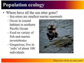
Static population patterns Geographic range – a population’s global distribution Fig. 50.2
Static population patterns Population size – the total number of individuals in a population Fig. 50.2
Static population patterns Density – the number of individuals per area Fig. 50.2
Static population patterns Dispersion – the pattern of spacing among individuals This map is NOT informative about dispersion! Fig. 50.2
Static population patterns Dispersion – the pattern of spacing among individuals Random – nearest neighbors are as near as predicted if all individuals were randomly placed within the focal boundaries Fig. 52.3c
Static population patterns Dispersion – the pattern of spacing among individuals Clumped (a.k.a. aggregated) – nearest neighbors are nearer, on average, than a random dispersion pattern would predict Fig. 52.3a
Static population patterns Dispersion – the pattern of spacing among individuals Uniform (a.k.a. regular) – nearest neighbors are farther away, on average, than a random dispersion pattern would predict Fig. 52.3b
Dynamic population patterns Geographic range, population size, density, dispersion can all change through time Fig. 52.19
Dynamic population patterns Consider population size; a population can grow, decline, or otherwise fluctuate Fig. 52.19
Demography The study of vital statistics that affect population size Fig. 52.19
Demography Life table – an age-specific summary of survival Table 52.1
Demography Life tables are often constructed by following the fate of a cohort Table 52.1
Demography Cohort – a group of individuals of the same age (or stage) Table 52.1
Demography Survivorship curve – a plot of the proportion out of a cohort alive at each age Figure 52.5
Demography Survivorship curve – a plot of the proportion out of a cohort alive at each age
Demography Reproductive table(a.k.a., fertility schedule) – age-specific reproductive rates Table 52.2
Demography Age structure – the relative number of individuals of each age in a population Figure 52.25
Demography Age structure – the relative number of individuals of each age in a population
Demography Age structure – the relative number of individuals of each age in a population
Demography Each population has its own characteristic vital rates(demographic parameters) The values of vital rates depend on the traits of the focal organisms…
For example… Coconut palms and kiwis produce a few, big offspring with high survivorship probabilities
For example… Dandelions and salmon produce many, tiny offspring with low survivorship probabilities
The traits that affect an organism’s vital rates, as well as the values of the vital rates themselves, comprise an organism’s life history vs.
Fitness costs and benefits shape life-history strategies vs.
Fitness costs and benefits are often balanced around life-history trade-offs Trait Y E.g., Seed size Trait X E.g., Seed number
Fitness costs and benefits are often balanced around life-history trade-offs Trait Y E.g., Number of lifetime reproductive episodes Iteroparity Semelparity (A single reproductive bout per lifetime) Trait X E.g., Number of offspring per reproductive episode
Fitness costs and benefits are often balanced around life-history trade-offs Current year reproduction vs. subsequent survival Fig. 52.7
Changes in population size (N) The following four processes can change the size of a population: 1. Birth 2. Death 3. Immigration 4. Emigration Fig. 52.2
Changes in population size (N) In a population closed to immigration and emigration: N = B - D t N the change in N for a given change in time = t B = the number of births D = the number of deaths
Changes in population size (N) We can also write the equation in terms of per capita birth and death rates: N = bN - dN t N the change in N for a given change in time = t b = the per capita birth rate d = the per capita death rate
Changes in population size (N) We can substitute r = (b - d) to give: N = rN t r = per capita growth rate If r > 0, population grows If r < 0, population declines If r = 0, population size remains the same
Changes in population size (N) We can substitute r = (b - d) to give: N = rN t For example… N2=1500 N1=1000 rN=500; r=0.5
Changes in population size (N) A population with unlimited resources would achieve its maximum growth rate: N = rmaxN t This is known as exponential growth
Changes in population size (N) Exponential growth is unlimited… Fig. 52.12
Changes in population size (N) An example of exponential growth:
Changes in population size (N) An example of near-exponential growth:
Changes in population size (N) An example of near-exponential growth:
Changes in population size (N) Real-world populations never continue growing exponentially indefinitely… Fig. 52.12
Changes in population size (N) Because many factors limit maximum population sizes, especially resources Fig. 52.12
Changes in population size (N) Carrying capacity (K) is the ceiling population size set by limited resources Fig. 52.12
Changes in population size (N) Logistic population growth describes a population that grows to carrying capacity Fig. 52.12
Changes in population size (N) An example of logistic growth:
Changes in population size (N) An example of near-logistic growth:
Changes in population size (N) An example of near-logistic growth: Fig. 52.13b
Changes in population size (N) The logistic equation incorporates a term that slows population change near K: N = rmaxN (K - N / K) t Fig. 52.11
Changes in population size (N) Density-dependent population change will tend to stabilize population size N = rmaxN (K - N / K) t Fig. 52.11
Changes in population size Density-dependent population change requires at least one density-dependent vital rate Fig. 52.14
4.0 10,000 3.8 3.6 Average number of seeds per reproducing individual (log scale) 1,000 3.4 Average clutch size 3.2 3.0 100 2.8 0 0 40 50 60 80 20 30 10 70 0 10 100 Seeds planted per m2 Density of females Changes in population size (N) Density-dependent population change requires at least one density-dependent vital rate Fig.52.15