Download
1 / 48
480 likes | 664 Views
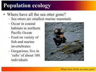
Population Ecology. Population Growth Models. A population is a group of individuals of a single species living in the same general geographic area Population density: the number of individuals per given area (# kangaroos/km 2 ). Patterns of Dispersion.

E N D
Population Ecology Population Growth Models
A population is a group of individuals of a single species living in the same general geographic area • Population density: the number of individuals per given area • (# kangaroos/km2)
Patterns of Dispersion • Clumped - most common. Due to optimum conditions, mating needs and/or predation strategy • Uniform - due to antagonist interactions. • Random - very uncommon.
Demography - study of vital statistics of a population, particularly birth and death rates • Survivorship curves plot the proportion of individuals alive at each age. • Three types of survivorship curves reflect important species differences in life history • Type I - low deaths rates during early and middle life. Humans and large mammals. • Type II - Constant death rate. Small mammals, invertebrates, lizards. • Type III - High death rates for young. Fish and invertebrates
Life Histories • There are trade-offs that each species makes between survival and frequency of reproduction, number of offspring produced and investment in parental care. • Life histories entail 3 basic variables: 1. When reproduction begins 2. How often the organism reproduces/Number of reproductive episodes per lifetime 3. How many offspring are produced during each reproductive episode/clutch size
Large Clutch Size • Benefits: lots of offspring • Tradeoff: small eggs or offspring, little energy to start life. • Typically with a Type III survivorship curve.
Small Clutch Size • Benefits: larger offspring, better chance of surviving to adulthood. • Tradeoff: fewer offspring • Typical with a Type I or II survivorship curve.
One Reproductive Episode • Benefit: can invest all of its energy into the production of offspring • Tradeoff: won’t live to reproduce again. • Also called semelparity • Salmon, Agave plants
Repeated Reproduction • Benefits: better chance of surviving to reproduce again, can possibly give care to offspring. • Tradeoff: not all of the energy goes to reproduction, some goes to growth and maintenance. • Also called iteroparity • Lizards,
Early Reproductive Age • Benefits: less chance of dying before reproductive age, shorter generation time. • Tradeoff: Less energy for maintenance and growth, reducing potential for large clutches in the future..
Later Reproductive Age • Benefit: Increase potential for future reproduction, older the female the larger the clutches. • Tradeoff: may die before first reproduction.
Ideal Reproductive Output • Early age • Large clutch • Reproduce many times • If survival rate for offspring is low, species will have one reproductive episode and produce many offspring. If the environment is more stable, species will generally have repeated offspring with smaller clutch sizes.
Two Life Histories • Opportunistic: based on the production of large numbers of offspring in a single reproductive event • Equilibrial: based on the repeated production of smaller number of better endowed offspring.
Opportunistic (r selected) • Benefit: large numbers, when conditions are favorable they can drastically increase in number. • Tradeoff: low survivorship, when conditions are poor many die without reproducing. • Typical of species taking over disturbed habitats.
Equilibrial (K selected) • Benefit: stronger offspring more likely to survive in adverse conditions. Less affected by environmental fluctuations. • Tradeoff: Fewer offspring, slow maturation. • Typical of terrestrial vertebrates.
Mathematical Growth Models • Are used to predict the number of organisms in a population over time. • Researchers can manipulate variables such as habitat destruction or harvesting to see their effects on a population.
Exponential Growth Model • When a population grows at the fastest rate possible for the species. • Occurs under ideal circumstances. • No restrictions on the abilities of individuals to harvest energy, grow, and reproduce.
Rate of Increase • Birthrate (b)- the number of births in a given year • Death rate (d) - the number of deaths in a given year. • Population (N)- the number of individuals in the population • r = (b-d)/N
Rate of Increase • The current population of deer mice in a field is 500. • The birthrate is approximately 25 per year. • The death rate is approximately 15 per year. • What is the Rate of Increase for the population?
Rate of Increase r = (25 – 15) / 500 r = .02 Rate of Increase = 2%
Expected Increase • To determine the number of new individuals in a population you multiply the rate of natural increase (r) by the current population size. I = r N
Expected Increase • After one year our mouse population will grow by how much?
Expected increase I = r N I = .02 * 500 I = 10 After one year the new population will by 510 deer mice!
Expected Increase • What will the population be after two years? I = .02 * 510 = 10.2 N(year 2) = 520.2 • What will the population be after 3 years?
More on Exponential Growth • In this model, population increases by an ever larger amount each year! • The resulting growth curve resembles a J-shape. • Species that exhibit this type of growth are described as r-selected species because their population growth rates may be close to their biotic potential.
Logistic Population Growth • Populations tend to have limits. • As populations grow more dense, resources become more scarce. • If the resources are not unlimited the population will not be able to grow exponentially for long.
Carrying Capacity • The maximum stable population size that a particular environment can support over a relatively long period of time. • Carrying capacity of a population depends on the species and the location. • Carrying capacity results from density dependent limiting factors such as food, water, shelter…
Logistic Model • The logistic model is a modification of the exponential model adding carrying capacity (K) into the equation. • This equation shows that the population growth rate decreases as the population increases or in other words the growth rate decreases as the population approaches carrying capacity. I = r ((K – N)/K) N **(K - N) / K = fraction that is still available for population growth
Logistic Growth Model • Consider a population with a carrying capacity of 200 and a current population of 150. What is the expected increase in population? I = r ((K – N)/K) N I = .1 ((200-150)/200)150 I = 3.75 **Without using the logistic growth model, the expected increase would be 15! • What about when the population reaches 180? I = r ((K – N)/K) N I = .1 ((200-180)/200)180 I = 1.8 **Without using the logistic growth model, the expected increase would be 18!
Logistic Growth Model • The equation results in a logistic S-shaped curve. • As the population reaches carrying capacity it begins to level off.
Logistic Growth Big Picture • The major biological implication of the logistic model is that increasing population density reduces the resources available for individual organisms and that resource limitation ultimately limits population growth!!!! • Some limitations, such as the Allee effect
Intraspecific competition • The logistic model depends on intraspecific competition: which is two animals of the same species competing for similar resources.
Density-Dependent Factors • Any factor is one that intensifies as the population increases in size • Negative Feedback! • Reduces birth rate and/or increases death rate • Examples: Competition for resources and territory, health, predation, build-up of waste products, and psychological factors
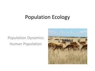
Population Dynamics • All populations undergo fluctuation due to complex environmental interactions. • Species that immagrate/emigrate can form metapopulations, making the study of populations even more complex! • Some populations undergo “boom-and-bust” cycles on a regular basis
Density-Independent Factors • Any factor that does not intensify with an increase in density.