Solution of linear system of equations

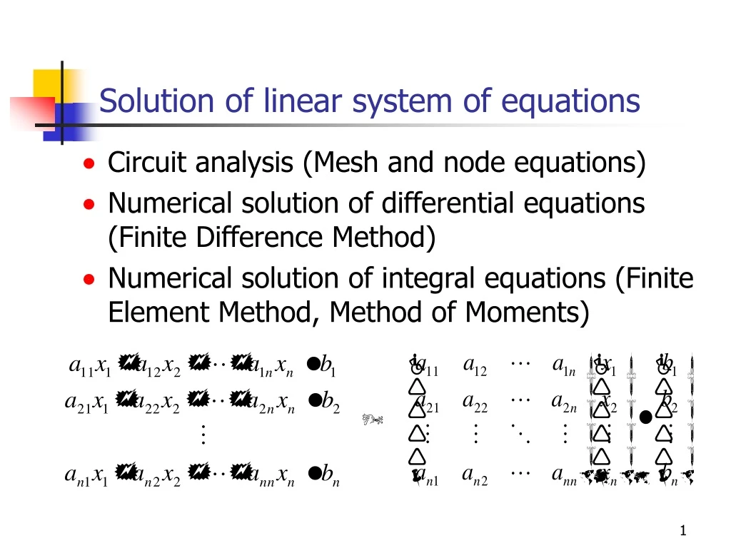
1.  Solution of linear system of equations • Circuit analysis (Mesh and node equations) • Numerical solution of differential equations (Finite Difference Method) • Numerical solution of integral equations (Finite Element Method, Method of Moments)

2. Consistency (Solvability) • The linear system of equations Ax=b has a solution, or said to be consistent IFF Rank{A}=Rank{A|b} • A system is inconsistent when Rank{A}<Rank{A|b} Rank{A} is the maximum number of linearly independent columns or rows of A. Rank can be found by using ERO (Elementary Row Oparations) or ECO (Elementary column operations). ERO# of rows with at least one nonzero entry ECO# of columns with at least one nonzero entry

3. Elementary row operations • The following operations applied to the augmented matrix [A|b], yield an equivalent linear system • Interchanges: The order of two rows can be changed • Scaling: Multiplying a row by a nonzero constant • Replacement: The row can be replaced by the sum of that row and a nonzero multiple of any other row.

4. An inconsistent example ERO:Multiply the first row with -2 and add to the second row Rank{A}=1 Then this system of equations is not solvable Rank{A|b}=2

5. Uniqueness of solutions • The system has a unique solution IFF Rank{A}=Rank{A|b}=n n is the order of the system • Such systems are called full-rank systems

6. Full-rank systems • If Rank{A}=n Det{A}  0  A is nonsingular so invertible Unique solution

7. Rank deficient matrices • If Rank{A}=m<n Det{A} = 0  A is singular so not invertible infinite number of solutions (n-m free variables) under-determined system Rank{A}=Rank{A|b}=1 Consistent so solvable

8.   Ill-conditioned system of equations • A small deviation in the entries of A matrix, causes a large deviation in the solution.

9. Ill-conditioned continued..... • A linear system of equations is said to be “ill-conditioned” if the coefficient matrix tends to be singular

10. Types of linear system of equations to be studied in this course • Coefficient matrix A is square and real • The RHS vector b is nonzero and real • Consistent system, solvable • Full-rank system, unique solution • Well-conditioned system

11. Solution Techniques • Direct solution methods • Finds a solution in a finite number of operations by transforming the system into an equivalent system that is ‘easier’ to solve. • Diagonal, upper or lower triangular systems are easier to solve • Number of operations is a function of system size n. • Iterative solution methods • Computes succesive approximations of the solution vector for a given A and b, starting from an initial point x0. • Total number of operations is uncertain, may not converge.

12.  Back substitution ERO Direct solution Methods • Gaussian Elimination • By using ERO, matrix A is transformed into an upper triangular matrix (all elements below diagonal 0) • Back substitution is used to solve the upper-triangular system

13. Pivotal element First step of elimination

14. Pivotal element Second step of elimination

15. Gaussion elimination algorithm For c=p+1 to n

16. Back substitution algorithm

17. Dominates Not efficient for different RHS vectors Operation count • Number of arithmetic operations required by the algorithm to complete its task. • Generally only multiplications and divisions are counted • Elimination process • Back substitution • Total

18. LU Decomposition A=LU Ax=b LUx=b Define Ux=y Ly=b Solve y by forward substitution ERO’s must be performed on b as well as A The information about the ERO’s are stored in L Indeed y is obtained by applying ERO’s to b vector Ux=y Solve x by backward substitution

19. LU Decomposition by Gaussian elimination There are infinitely many different ways to decompose A. Most popular one: U=Gaussian eliminated matrix L=Multipliers used for elimination Compact storage: The diagonal entries of L matrix are all 1’s, they don’t need to be stored. LU is stored in a single matrix.

20. Operation count Done only once • A=LU Decomposition • Ly=b forward substitution • Ux=y backward substitution • Total • For different RHS vectors, the system can be efficiently solved.

21. Pivoting • Computer uses finite-precision arithmetic • A small error is introduced in each arithmetic operation, error propagates • When the pivotal element is very small, the multipliers will be large. • Adding numbers of widely differening magnitude can lead to loss of significance. • To reduce error, row interchanges are made to maximise the magnitude of the pivotal element

22. Example: Without Pivoting 4-digit arithmetic Loss of significance

23. Example: With Pivoting

24. Eliminated part Pivotal row Pivotal column Pivoting procedures

25. Row pivoting • Most commonly used partial pivoting procedure • Search the pivotal column • Find the largest element in magnitude • Then switch this row with the pivotal row

26. Interchange these rows Largest in magnitude Row pivoting

27. Largest in magnitude Interchange these columns Column pivoting

28. Interchange these rows Largest in magnitude Interchange these columns Complete pivoting

29. Row Pivoting in LU Decomposition • When two rows of A are interchanged, those rows of b should also be interchanged. • Use a pivot vector. Initial pivot vector is integers from 1 to n. • When two rows (i and j) of A are interchanged, apply that to pivot vector.

30. Modifying the b vector • When LU decomposition of A is done, the pivot vector tells the order of rows after interchanges • Before applying forward substitution to solve Ly=b, modify the order of b vector according to the entries of pivot vector

31. LU decomposition algorithm with row pivoting Column search for maximum entry Interchaning the rows Updating L matrix For c=k+1 to n Updating U matrix

32. Column search: Maximum magnitude second row Interchange 1st and 2nd rows Example

33. Multipliers (L matrix) Example continued... Eliminate a21 and a31 by using a11 as pivotal element A=LU in compact form (in a single matrix)

34. Column search: Maximum magnitude at the third row Interchange 2nd and 3rd rows Example continued...

35. Multipliers (L matrix) Example continued... Eliminate a32 by using a22 as pivotal element

36. Example continued... A’x=b’ LUx=b’ Ux=y Ly=b’

37. Ly=b’ Forward substitution Ux=y Backward substitution Example continued...

38. Gauss-Jordan elimination • The elements above the diagonal are made zero at the same time that zeros are created below the diagonal

39. Gauss-Jordan Elimination • Almost 50% more arithmetic operations than Gaussian elimination • Gauss-Jordan (GJ) Elimination is prefered when the inverse of a matrix is required. • Apply GJ elimination to convert A into an identity matrix.

40. Different forms of LU factorization • Doolittle form Obtained by Gaussian elimination • Crout form • Cholesky form

41. Crout form • First column of L is computed • Then first row of U is computed • The columns of L and rows of U are computed alternately

42. 2 4 6 1 3 5 7 Crout reduction sequence An entry of A matrix is used only once to compute the corresponding entry of L or U matrix So columns of L and rows of U can be stored in A matrix

43. Cholesky form • A=LDU (Diagonals of L and U are 1) • If A is symmetric L=UT  A= UT DU= UT D1/2D1/2U U’= D1/2U  A= U’T U’ This factorization is also called square root factorization. Only U’ need to be stored

44. Solution of Complex Linear System of Equations Cz=w C=A+jB Z=x+jy w=u+jv (A+jB)(x+jy)=(u+jv) (Ax-By)+j(Bx+Ay)=u+jv Real linear system of equations

45. Large and Sparse Systems • When the linear system is large and sparse (a lot of zero entries), direct methods become inefficient due to fill-in terms. • Fill-in terms are those which turn out to be nonzero during elimination Fill-in terms Elimination

46. Sparse Matrices • Node equation matrix is a sparse matrix. • Sparse matrices are stored very efficiently by storing only the nonzero entries • When the system is very large (n=10,000) the fill-in terms considerable increases storage requirements • In such cases iterative solution methods should be prefered instead of direct solution methods