Solution of Linear State- Space Equations
Solution of Linear State- Space Equations. Outline. • Laplace solution of linear state-space equations . • Leverrier algorithm. • Systematic manipulation of matrices to obtain the solution. Linear State-Space Equations. 1. Laplace transform to obtain their solution x ( t ) .

Solution of Linear State- Space Equations
E N D
Presentation Transcript
Outline • Laplace solution of linear state-space equations. • Leverrieralgorithm. • Systematic manipulation of matrices to obtain the solution.
Linear State-Space Equations 1. Laplace transform to obtain their solution x(t). 2. Substitute in the output equation to obtain the output y(t).
Laplace Transformation • Multiplication by a scalar (each matrix entry). • Integration (each matrix entry).
State-transition Matrix • LTI case φ (t − t0) = matrix exponential • Zero-input response: multiply by state transition matrix to change the system state from x(0) to x(t). • State-transition matrix for time-varying systems φ (t, t0) – Not a matrix exponential (in general). – Depends on initial & final time (not difference between them).
Example 7.7 x1 = angular position, x2 = angular velocity x3 = armature current. Find: a)The state transition matrix. b)The response due to an initial current of 10 mA. c)The response due to a unit step input. d)The response due to the initial condition of (b) together with the input of (c)
Remarks • Operations available in hand-held calculators (matrix addition & multiplication, matrix scalar multiplication). • Trace operation ( not available) can be easily 22 p ) y programmed using a single repetition loop. • Initialization and backward iteration starts with: Pn-2 = A + an-1 In an-2 = − ½ tr{Pn-2 A}
Example 7.8 Calculate the matrix exponential for the state matrix of Example 7.7 using the Leverrier algorithm.