Download
1 / 42
420 likes | 630 Views
Hardware Assisted Solution of Huge Systems of Linear Equations. Adi Shamir Computer Science and Applied Math Dept The Weizmann Institute of Science Joint work with Eran Tromer Hebrew University, 6/3/06. Cryptanalysis is Evil. A simple mathematical proof:

E N D
Hardware Assisted Solution ofHuge Systems of Linear Equations Adi Shamir Computer Science and Applied Math Dept The Weizmann Institute of Science Joint work with Eran Tromer Hebrew University, 6/3/06
Cryptanalysis is Evil • A simple mathematical proof: • The definition of throughput cost implies that cryptanalysis = time x money • Since time = money, cryptanalysis = money2 • Since money is the root of evil, money25=evil • Consequently, cryptanalysis = evil
Cryptanalysis is Useful: • Raises interesting mathematical problems • Requires highly optimized algorithms • Leads to new computer architectures • Motivates the development of new technologies • Stretches the limits on what’s doable
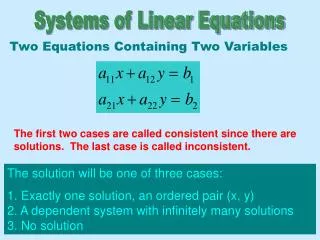
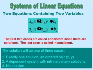
Motivation for this Talk: Integer Factorization and Cryptography multiplication is easy • RSA uses n as the public key and p,q as the secret key in encrypting and signing messages • The size of the public key n determines the efficiency and the security of the scheme Large primes p,q Product n=p£q factorization is hard
Factorization Records: • A 256 bit key used by French banks in 1980’s • A 512 bit key factored in 1999 • A 667 bit (200 digit) key factored in 2005 • The big challenge: factoring 1024 bit keys
Improved Factorization ResultsCan be derived from: • New algorithms for standard computers (which are better than the Number Field Sieve) • Non-conventional computation models (unlimited word length, quantum computers) • Faster standard devices (Moore’s law) • New implementations of known algorithms on special purpose hardware (wafer scale integration, optoelectronics, …)
The Basic Idea of the Number Field Sieve (NFS) Factoring Algorithm: To factor n: • Find “random” r1,r2such that r12 r22 (mod n) • Hope that gcd(r1-r2,n) is a nontrivial factor of n. How? • Let f1(a) = a2 mod n These values are squares mod n, but not over Z • Find a nonempty set S½Z such thatthe product of the values of f1(a) for a2S is a square over the integers • This gives us the two “independent” representations r12 r22 (mod n)
Some Technical Details: How to find Ssuch that is a square? • Consider all the primes smaller than some bound B, and find many integers a for which f1(a) isB-smooth. • For each such a, represent the factorization of f1(a) as a vector of b exponents: f1(a)=2e1 3e2 5e3 7e4 L a (e1,e2,...,eb) • Once b+1 such vectors are found, find a dependency modulo 2 among them. That is, find S such that=2e1 3e2 5e3 7e4 L where the ei are all even. Sieving step Matrix step
A Simple example: We want to find a subset Ssuch that is a square Look at the factorization of smooth f1(a) which factor completely into a product of small primes: This is a square, because all exponents are even.
The Matrix Step in the Factorization of 1024 Bit Numbers can thus be Reduced to the following problem: Find a nonzero x satisfying Ax=0 over GF(2) where: • A is huge (#rows/columns larger than 230 ) • A is sparse (#1’s per row less than 100) • A is “random” (with no usable structure) • The algorithm can occasionally fail
Solving linear equations and finding kernel vectors are computationally equivalent problems: • Let A’ be a non-singular matrix. • Let A be the singular matrix defined by adding b as a new column and adding zeroes as a new row in A’. • Consider any nonzero kernel vector x satisfying Ax=0. The last entry of x cannot be zero, so we can use the other entries x’ of x to describe b as a linear combination of the columns of A’, thus solving A’x’=b.
Solving linear equations and finding kernel vectors are computationally equivalent problems:
Standard Equation Solving Techniques Are Impractical: • Elimination and factoring techniques quickly fill up the sparse initial matrix • Approximation techniques do not work mod 2 • Many specialized techniques do not work for random matrices • Random access to matrix elements is too expensive • Parallel processing is impractical unless restricted to 2D grids with local communication between neighbors
Practical limits on what we can do: • We can use linear space to store the original sparse matrix (with 100x230“1” entries), along with several dense vectors, but not the quadratic number of entries in a dense matrix of this size (with260entries) • We can use a quadratic time algorithm (260steps) but not a cubic time algorithms (290steps) to solve the linear algebra problem • We have to use special purpose hardware and highly optimized algorithms
Wiedemann’s Algorithm to find a vector u in the kernel of a singular A: • Theorem: Let p(x) be the characteristic polynomial of the matrix A. Then p(A)=0. • Lemma: If A is singular, 0 is a root of p(x), and thus p(x)=xq(x). • Corollary: Aq(A)=p(A)=0, and thus for any vector v, u=q(A)v is in the kernel of A.
Wiedemann’s Algorithm to find a vector u in the kernel of a singular A: • We have thus reduced the problem of finding a kernel vector of a sparse A into the problem of finding its characteristic polynomial. • The basic idea: Consider the infinite sequence of powers of A:A,A2,A3,...,Ad,...(mod 2). • If A has dimension dxd, we know that its characteristic polynomial has degree at most d, and thus the matrices in any window of length d satisfy the same linear recurrence relation mod 2.
Wiedemann’s Algorithm to find a vector u in the kernel of a singular A: • The matrices are too large and dense, so we cannot compute and store them. • To overcome this problem, pick a random vectorvand compute the first bit of each vectorAv,A2v,A3v,...,Adv,...(mod 2). • These bits satisfy the same linear recurrence relation of size d(mod 2).
Wiedemann’s Algorithm to find a nonzero vector in the kernel of a singular A: • Given a binary sequence of bits length d, we can find their shortest linear recurrence by using the Berlekamp-Massey algorithm, which runs in quadratic time using linear space. • To compute the sequence of vectorsAv,A2v,A3v,...,Adv,...(mod 2), we have to repeatedly compute the product of the sparse matrix A by the previous dense vector. • Each matrix-vector product requires linear time and space. Since we have to compute d such products but retain only the top bit from each one of them, the whole computation requires quadratic time and linear space.
How to Perform the Sparse Matrix / Dense Vector Products Daniel Bernstein’s observations (2001): • On a single-processor computer, storage dominates cost but is poorly utilized. • Sharing the input among multiple processors can lead to collisions, propagation delays. • Solution: use a mesh-based architecture with a small processor attached to each memory cell, and use a mesh sorting algorithm to perform the matrix/vector multiplications.
Σ Matrix-by-vector multiplication X = (mod 2)
Is the mesh sorting idea optimal? • The fastest known mesh sorting algorithm for a mxm mesh requires about 3m steps, but it is too complicated to implement on simple processors. • Bernstein used the Schimmler mesh sorting algorithm three times to complete each matrix-vector product. For a mxm matrix, this requires about 24m steps. • We proposed to replace the mesh sorting by mesh routing, which is both simpler and faster. We use only one full routing, which requires 2m steps.
A routing-based circuit for the matrix step[Lenstra,Shamir,Tomlinson,Tromer 2002] Model: two-dimensional mesh, nodes connected to ·4 neighbours. Preprocessing: load the non-zero entries of A into the mesh, one entry per node. The entries of each column are stored in a square block of the mesh, along with a “target cell” for the corresponding vector bit.
Operation of the routing-based circuit To perform a multiplication: • Initially the target cells contain the vector bits. These are locally broadcast within each block(i.e., within the matrix column). • A cell containing a row index ithat receives a “1” emits an value(which corresponds to a at row i). • Each value is routed to thetarget cell of the i-th block(which is collecting ‘s for row i). • Each target cell counts thenumber of values it received. • That’s it! Ready for next iteration.
How to perform the routing? If the original sparse matrix A has size dxd, we have to fold the d vector entries into a mxm mesh where m=sqrt(d). Routing dominates cost, so the choice of algorithm (time, circuit area) is critical. There is extensive literature about mesh routing. Examples: • Bounded-queue-size algorithms • Hot-potato routing • Off-line algorithms None of these are ideal.
1 2 4 3 Clockwise transposition routing on the mesh • One packet per cell. • Only pairwise compare-exchange operations ( ). • Compared pairs are swapped according to the preference of the packet that has the farthestto go along this dimension. • Very simple schedule, can be realized implicitly by a pipeline. • Pairwise annihilation. • Worst-case: m2 • Average-case: ? • Experimentally:2m steps suffice for random inputs – optimal. • The point: m2 values handled in time O(m). [Bernstein]
Comparison to Bernstein’s design 1/12 • Time: A single routing operation (2m steps)vs. 3 sorting operations (8m steps each). • Circuit area: • Only the move; the matrix entries don’t. • Simple routing logic and small routed values • Matrix entries compactly stored in DRAM (~1/100 the area of “active” storage) 1/3
Further improvements 1/7 • Reduce the number of cells in the mesh (for small μ, decreasing #cells by a factor of μ decreases throughput cost by ~μ1/2) • Use Coppersmith’s block Wiedemann • Execute the separate multiplication chains of block Wiedemann simultaneously on one mesh (for small K, reduces cost by ~K) Compared to Bernstein’s original design, this reduces the throughput cost by a constant factor 1/6 1/15 of 45,000.
Does it always work? • We simulated the algorithm thousands of time with large random mxm meshes, and it always routed the data correctly within 2m steps • We failed to prove this (or any other) upper bound on the running time of the algorithm. • We found a particular input for which the routing algorithm failed by entering a loop.
Hardware Fault tolerance • Any wafer scale design will contain defective cells. • Cells found to be defective during the initial testing can be handled by modifying the routing algorithm.
Algorithmic fault tolerance • Transient errors must be detected and corrected as soon as possible since they can lead to totally unusable results. • This is particularly important in our design, since the routing is not guaranteed to stop after 2m steps, and packets may be dropped
How to detect an error in the computation of AxV (mod 2)? The original matrix-vector product:
How to detect an error in the computation of AxV (mod 2)? Sum of some matrix rows: Check bit
Problems with this solution: • If the new test vector at the bottom is the sum mod 2 of few rows, it will remain sparse but have extremely small chance of detecting a transient error in one of the output bits • If the new test vector at the bottom is the sum mod 2 of a random subset of rows, it will become dense, but still miss errors with constant probability
Problems with this solution: • To reduce the probability of missing an error to a negligible value, we can add hundreds of dense test vectors derived from independent random subsets of the rows of the matrix. • However, in this case the cost of the checking dominates the cost of the actual computation.
Our new solution: • We add only one test vector, which adds only 1% to the cost of the computation, and still get negligible probability of missing transient errors • We achieve it by using the fact that in Weidemann’s algorithm we compute all the products • V1=AV, V2=A2V, V3=A3V, …Vi=AiV,…VD=ADV
Our new solution: • We choose a random row vector R, and precompute (on a reliable machine) the row vector W=RAkfor some small k (e.g., k=200). • We add to the matrix the two row vectors W and R as the only additional test vectors. Note that these vectors are no longer the sum of subsets of rows of the matrix A.
Our new solution: • Consider now the following equation, which is true for all i: Vi+k=Ai+kV=AkAiV=AkVi • Multiplying it on the left with R, we get that for all i: RVi+k=RAkVi=WVi • Since we added the two vectors R and W to the matrix, we get for each vector Vi the products RViand WVi , which are two bits
Our new solution: • We store the computed values of WVi in a short shift register of length k=200, and compare it after a delay k with the computed value of RVi+k • We periodically store the current vector Vi (say, once a day) in an off-line storage. If any one of the consistency tests fails, we stop the computation, test for faulty components, and restart from the last good Vi
Why does it catch transient errors with overwhelming probability? • Assume that at step i the algorithm computed the erroneous Vi ‘=Vi +E and that all the computations before and after step i were correct (wrt the wrong Vi ‘) • Due to the linearity of the computation, for any j>0: V ’i+j=AjV ’i=Aj(Vi+E)=AjVi+AjE=Vi+j+AjE and thus the difference between the correct and erroneous Vi develops as AjE from time i onwards
Why does it catch transient errors with overwhelming probability? • Each test checks whether W(AjE)=0 for some j<k • Since the matrix A generated by the number field sieve is random looking, its first k=200 powers are likely to be random and dense, and thus each test has an independent probability of 0.5 to fail. First error detection No more detectableerrors