Download
1 / 44
460 likes | 947 Views
Learn about image enhancement in the spatial domain, including grey level transformations, histogram processing, spatial filtering, and combining enhancement methods for improved image quality. Explore various methods to enhance image contrast and clarity.

E N D
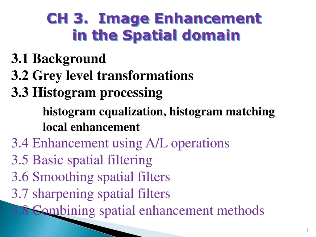
CH 3. Image Enhancement in the Spatial domain 3.1 Background 3.2 Grey level transformations 3.3 Histogram processing histogramequalization, histogram matching local enhancement 3.4 Enhancement using A/L operations 3.5 Basic spatial filtering 3.6 Smoothing spatial filters 3.7 sharpening spatial filters 3.8 Combining spatial enhancement methods
3.1 Background • Why image enhancement ? • 1. processing an images so that the result is more suitable than the original image for a SPECIFIC application. • 2. Providing `better' input for other automated image processing techniques. • Two approaches • - Spatial domain methods: • operate directly on pixels • - Frequency domain methods: • operate on the Fourier transform of an image
3.1 Background • What is spatial domain? • - it refers to the aggregated of pixels composing an image. • Spatial domain processes will be denoted by the expression • g(x,y)=T[f(x,y)] • where f(x,y) is the input image, g(x,y) is the processed image (output image), and T is an operator of f
Background Gray-level transformation functions for contrast Enhancement.
3.2 Gray-Level Transformations • Some basic gray-level transformations:- • Three basic types of functions (Fig. 3.3) used for • image enhancement: • Image negative transformations • Log transformations • Power-law transformations
Gray-Level Transformations • Image negative transform: s = T(r) • obtained by using the negative transformation • s = L-1 – r e.g. Input=10, output=255-10 • - produces the equivalent of a photographic negative • - suited for enhancing white or gray detail embedded • in dark regions of an image.
3.2.2 Log transformations • Log transformations: s = c log(1+r) • - Expand the values of dark pixels while compressing the high-level values • - Compress the dynamic range of images with large variations
3.2.2 Log transformations LOG TRANFORM IMAGE INPUT IMAGE
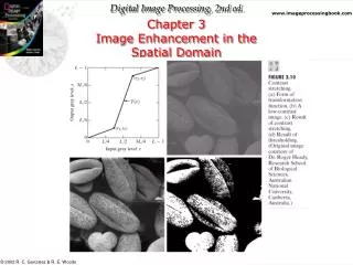
3.2.4 Piecewise-linear transform functions • Advantage: its form can be arbitrary complex over the previous functions • Disadvantage: require considerably more user input • Contrast stretching • - One of the simplest piecewise function • - Increase the dynamic range of the gray levels in the image • - A typical transformation: control the shape of the transformation • e.g. if r1 = r2, s1=0 and s2=L-1 threshold function
3.2.4 Piecewise-linear transform functions • Gray-level slicing • - Highlight a specific range of gray levels • - Display a high value for all gray levels in the range of interest and a low value for all other gray levels : • produce a binary image (Fig. 3.11(a)) • - Preserving background (Fig. 3.11(b))
Bit-plane slicing • Bit-plane slicing • - Suppose that each pixel in an image is represented by 8 bits. • - Imagine that the image is composed of eight 1-bit planes, ranging from bit-plane 0 (the least significant bit) to bit-plane 7 (the most significant bit).
Bit-plane slicing Original Image Bit-plane 6 Bit-plane 1 Bit-plane 7 Bit-plane 4
3.3 Histogram Processing • Types of processing: • Histogram Equalization • Histogram Matching(Specification) • Local Enhancement
3.3.1 Histogram equalization Histogram Equalization: - produce a level s for every pixel value r in the input image. - the transformation function T(r) satisfies the following: (a) T(r) is single-valued and monotonically increasing in the interval 0 ≤ r ≤ 1; and (b) 0 ≤ T(r) ≤ 1 for 0 ≤ r ≤ 1
3.3.1 Histogram equalization • n = total # of pixel, nk = #of pixel having gray-level k • Probability of occurrence of gray-level rk • Pr(rk) = nk/n • Cumulative Distribution Function(CDF) • - Histogram equalization(HE) results are similar to contrast stretching - the advantage: HE automatically determines a transformation function to produce a new image with a uniform histogram.
3.3.2 Histogram matching/specification • Enhancement based on a uniform histogram is not always the best approach • It is useful sometimes to specify the shape of the histogram that we wish to have • Suitable for interactive image enhancement • Difficulty--building a meaningful histogram • The procedure for histogram matching (Page 99)
3.3.2 Histogram matching/specification - Specify the desired density function and obtain the transformation function G(z): pz: specified desirable PDF for output -Find z by using s = v
3.3.3 Histogram Local Enhancement • Normally, transformation function based on the content of an entire image. • Some cases it is necessary to enhance details over small areas in an image. • The histogram processing techniques are easily adaptable to local enhancement.
3.3.4 Histogram Statistics for Image Enhanc. Contrast manipulation using local statistics (the mean and variance) is useful for images where part of the image is acceptable, but other parts may contain hidden features of interest.
3.3.4 Histogram Statistics for Image Enhanc. Enhanced Image Original Image
Summary • 3.1 Background • Why enhancement? Specific app. • Spatial/freq. domain • 3.2 Grey level transformations • Image negatives • Log transformations • Power-law transformations • Piecewise-linear transformation function • Contrast stretching, gray-level slicing, bit-plane-slicing • 3.3 Histogram processing • histogramequalization, • histogram matching • local enhancement t