Digital Image Processing Image Enhancement in Spatial Domain
370 likes | 952 Views
Digital Image Processing Image Enhancement in Spatial Domain. Dr. Abdul Basit Siddiqui. Image Sampling and Quantization. To create a digital image, we need to convert the continuous sensed data into digital form --> this involves sampling and quantization

Digital Image Processing Image Enhancement in Spatial Domain
E N D
Presentation Transcript
Digital Image ProcessingImage Enhancement in Spatial Domain Dr. Abdul Basit Siddiqui
Image Sampling and Quantization • To create a digital image, we need to convert the continuous sensed data into digital form --> this involves sampling and quantization • Digitizing the coordinate values is called sampling • Digitizing the amplitude values is called quantization ---> see Fig. 2.16 in the textbook • In practice, the method of sampling is determined by the sensor arrangement used to generate the image • The quality of a digital image is determined by the number of samples and the number of gray levels
Spatial resolution and intensity resolution • Sampling is the principal factor defining the spatial resolution of an image, and quantization is the principal factor defining the intensity resolution • Spatial resolution - number of rows and columns for example: 128 x128, 256 by 256, etc.; -->see Figs. 2.19 and 2.20 • Intensity resolution - number of gray levels for example: 8 bits, 16 bits, etc.; --->see Fig. 2.21
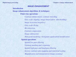
Image Enhancement Process an image to make the result more suitable than theoriginal image for a specific application –Image enhancement is subjective (problem /application oriented) Image enhancement methods: Spatial domain: Direct manipulation of pixel in an image (on the image plane) Frequency domain: Processing the image based on modifying the Fourier transform of an image Many techniques are based on various combinations of methods from these two categories
Basic Concepts Spatial domain enhancement methods can be generalized as g(x,y)=T[f(x,y)] f(x,y): input image g(x,y): processed (output) image T[*]: an operator on f (or a set of input images), defined over neighborhood of (x,y) Neighborhood about (x,y): a square or rectangular sub-image area centered at (x,y)
Point Processes • Point processes are the simplest of basic image processing operations. • A point operation takes a single input image into a single output image in such a way that each output pixel's gray level depends only upon the gray level of the corresponding input pixel. • Thus, a point operation cannot modify the spatial relationships within an image. • Point operations transform the gray scale of an image.
Point Processes • Linear and nonlinear point operations • Examples: • Contrast Stretching • Image Negatives • Intensity-level Slicing • Bit-plane Slicing • Other Intensity Transformations • Histogram Equalization
Basic Concepts g(x,y) = T [f(x,y)] Pixel/point operation: Neighborhood of size 1x1: g depends only on f at (x,y) T: a gray-level/intensity transformation/mapping function Let r = f(x,y) s = g(x,y) r and s represent gray levels of f and g at (x,y) Then s = T(r) Local operations: g depends on the predefined number of neighbors of f at (x,y) Implemented by using mask processing or filtering Masks (filters, windows, kernels, templates) : a small (e.g. 3×3) 2-D array, in which the values of the coefficients determine the nature of the process
Common Pixel Operations • Image Negatives • Log Transformations • Power-Law Transformations
Image Negatives • Reverses the gray level order • For L gray levels the transformation function is s =T(r) = (L - 1) - r
Image Scaling s =T(r) = a.r(a is a constant)
Log Transformations Function ofs = cLog(1+r)
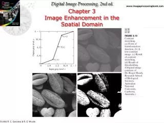
Log Transformations Properties of log transformations –For lower amplitudes of input image the range of gray levels is expanded –For higher amplitudes of input image the range of gray levels is compressed Application: • This transformation is suitable for the case when the dynamic range of a processed image far exceeds the capability of the display device (e.g. display of the Fourier spectrum of an image) • Also called “dynamic-range compression / expansion”
Power-Law Transformation For γ < 1: Expands values of dark pixels, compress values of brighter pixels For γ > 1: Compresses values of dark pixels, expand values of brighter pixels If γ=1 & c=1: Identity transformation (s = r) A variety of devices (image capture, printing, display) respond according to power law and need to be corrected Gamma (γ) correction The process used to correct the power-law response phenomena
Histogram • Gray level histogram of an image - a function showing for each gray level the number of • pixels in the image that have that gray level; it is simply a bar graph of the pixel intensities
Histogram • Histogram gives us a convenient, easy-to-read representation of concentration of pixels versus intensity in an image • Dynamic range - an range of intensity values that occur in an image • Contrast stretching - if image has low-dynamic range; low-dynamic range can result from poor illumination, lack of dynamic range in imaging sensor, wrong setting of the sensor parameters, etc. • Compression of dynamic range - if the dynamic range of the image far exceeds the capability of the display device
Histogram Equalization • Images with poor intensity distributions can often be enhanced with histogram equalization <-- point process • The goal is to obtain a uniform histogram • • Histogram equalization will not flatten a histogram; if a histogram has peaks and valleys it will still have them after equalization - they will be shifted and spread over the entire range of image intensities • Works best on images with fine details in darker regions • Use it carefully - good images can be often degraded by histogram equalization