Chapter 3 Image Enhancement in the Spatial Domain

1. Chapter 3 Image Enhancement in the Spatial Domain

2. The spatial domain: The imageplane For a digital image is a Cartesian coordinate system of discrete rows and columns. At the intersection of each row and column is a pixel. Each pixel has a value, which we will call intensity. The frequency domain: A (2-dimensional) discrete Fourier transform of the spatial domain We will discuss it in chapter 4. Enhancement: To “improve” the usefulness of an image by using some transformation on the image. Often the improvement is to help make the image “better” looking, such as increasing the intensity or contrast. Image Enhancement in the Spatial Domain

3. A mathematical representation of spatial domainenhancement: where f(x, y): the input image g(x, y): the processed image T: an operator on f, defined over some neighborhood of (x, y) Background

4. Gray-level Transformation

5. Some Basic Gray Level Transformations

6. Let the range of gray level be [0, L-1], then Image Negatives

7. Log Transformations where c : constant

8. Power-Law Transformation where c, : positive constants

9. Power-Law Transformation Example 1: Gamma Correction

10. Power-Law Transformation Example 2: Gamma Correction

11. Power-Law Transformation Example 3: Gamma Correction

12. Piecewise-Linear Transformation Functions Case 1: Contrast Stretching

13. Piecewise-Linear Transformation Functions Case 2:Gray-level Slicing Result of using the transformation in (a) An image

14. Bit-plane slicing: It can highlight the contribution made to total image appearance by specific bits. Each pixel in an image represented by 8 bits. Image is composed of eight 1-bit planes, ranging from bit-plane 0 for the least significant bit to bit plane 7 for the most significant bit. Piecewise-Linear Transformation Functions Case 3:Bit-plane Slicing

15. Piecewise-Linear Transformation Functions Bit-plane Slicing: A Fractal Image

16. Piecewise-Linear Transformation Functions Bit-plane Slicing: A Fractal Image 7 6 3 4 5 2 1 0

17. Histogram Processing

18. Histogram Processing

19. Histogram Equalization • Histogram equalization: • To improve the contrast of an image • To transform an image in such a way that the transformed image has a nearly uniform distribution of pixel values • Transformation: • Assume r has been normalized to the interval [0,1], with r = 0 representing black and r = 1 representing white • The transformation function satisfies the following conditions: • T(r) is single-valued and monotonically increasing in the interval

20. For example: Histogram Equalization

21. Histogram Equalization • Histogram equalization is based on a transformation of the probability density function of a random variable. • Let pr(r) and ps(s) denote the probability density function of random variable r and s, respectively. • If pr(r) and T(r) are known, then the probability density function ps(s) of the transformed variable s can be obtained • Define a transformation function where w is a dummy variable of integration and the right side of this equation is the cumulative distribution function of random variable r.

22. Histogram Equalization • Given transformation function T(r), ps(s) now is a uniform probability density function. • T(r) depends on pr(r), but the resulting ps(s) always is uniform.

23. Histogram Equalization • In discrete version: • The probability of occurrence of gray level rk in an image is n : the total number of pixels in the image nk : the number of pixels that have gray level rk L : the total number of possible gray levels in the image • The transformation function is • Thus, an output image is obtained by mapping each pixel with level rk in the input image into a corresponding pixel with level sk.

24. Histogram Equalization

25. Histogram Equalization

26. Transformation functions (1) through (4) were obtained form the histograms of the images in Fig 3.17(1), using Eq. (3.3-8). Histogram Equalization

27. Histogram matching is similar to histogram equalization, except that instead of trying to make the output image have a flat histogram, we would like it to have a histogram of a specified shape, say pz(z). We skip the details of implementation. Histogram Matching

28. The histogram processing methods discussed above are global, in the sense that pixels are modified by a transformation function based on the gray-level content of an entire image. However, there are cases in which it is necessary to enhance details over small areas in an image. Local Enhancement global local original

29. Moments can be determined directly from a histogram much faster than they can from the pixels directly. Let r denote a discrete random variable representing discrete gray-levels in the range [0,L-1], and p(ri) denote the normalized histogram component corresponding to the ith value of r, thenthe nth moment of r about its mean is defined as where m is the mean value of r For example, the second moment (also the variance of r) is Use of Histogram Statistics for Image Enhancement

30. Two uses of the mean and variance for enhancement purposes: The global mean and variance (global means for the entire image) are useful for adjusting overall contrast and intensity. The mean and standard deviation for a local region are useful for correcting for large-scale changes in intensity and contrast. ( See equations 3.3-21 and 3.3-22.) Use of Histogram Statistics for Image Enhancement

31. Use of Histogram Statistics for Image Enhancement Example: Enhancement based on local statistics

32. Use of Histogram Statistics for Image Enhancement Example: Enhancement based on local statistics

33. Use of Histogram Statistics for Image Enhancement Example: Enhancement based on local statistics

34. Two images of the same size can be combined using operations of addition, subtraction, multiplication, division, logical AND, OR, XOR and NOT. Such operations are done on pairs of their corresponding pixels. Often only one of the images is a real picture while the other is a machine generated mask. The mask often is a binary image consisting only of pixel values 0 and 1. Example: Figure 3.27 Enhancement Using Arithmetic/Logic Operations

35. AND OR Enhancement Using Arithmetic/Logic Operations

36. Image Subtraction Example 1

37. When subtracting two images, negative pixel values can result. So, if you want to display the result it may be necessary to readjust the dynamic range by scaling. Image Subtraction Example 2

38. Image Averaging • When taking pictures in reduced lighting (i.e., low illumination), image noise becomes apparent. • A noisy image g(x,y) can be defined by where f (x, y): an original image : the addition of noise • One simple way to reduce this granular noise is to take several identical pictures and average them, thus smoothing out the randomness.

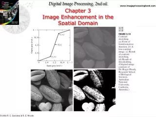
39. Figure 3.30 (a): An image of Galaxy Pair NGC3314. Figure 3.30 (b): Image corrupted by additive Gaussian noise with zero mean and a standard deviation of 64 gray levels. Figure 3.30 (c)-(f): Results of averaging K=8,16,64, and 128 noisy images. Noise Reduction by Image Averaging Example: Adding Gaussian Noise

40. Figure 3.31 (a): From top to bottom: Difference images between Fig. 3.30 (a) and the four images in Figs. 3.30 (c) through (f), respectively. Figure 3.31 (b): Corresponding histogram. Noise Reduction by Image Averaging Example: Adding Gaussian Noise

41. Basics of Spatial Filtering • In spatial filtering (vs. frequency domain filtering), the output image is computed directly by simple calculations on the pixels of the input image. • Spatial filtering can be either linear or non-linear. • For each output pixel, some neighborhood of input pixels is used in the computation. • In general, linear filtering of an image f of size MXN with a filter mask of size mxn is given by where a=(m-1)/2 and b=(n-1)/2 • This concept called convolution. Filter masks are sometimes called convolution masks or convolution kernels.

42. Basics of Spatial Filtering

43. Nonlinear spatial filtering usually uses a neighborhood too, but some other mathematical operations are use. These can include conditional operations (if …, then…), statistical (sorting pixel values in the neighborhood), etc. Because the neighborhood includes pixels on all sides of the center pixel, some special procedure must be used along the top, bottom, left and right sides of the image so that the processing does not try to use pixels that do not exist. Basics of Spatial Filtering

44. Smoothing linear filters Averaging filters (Lowpass filters in Chapter 4)) Box filter Weighted average filter Weighted average Box filter Smoothing Spatial Filters

45. Smoothing Spatial Filters • The general implementation for filtering an MXN image with a weighted averaging filter of size mxn is given by where a=(m-1)/2 and b=(n-1)/2

46. Smoothing Spatial Filters Image smoothing with masks of various sizes

47. Smoothing Spatial Filters Another Example

48. Order-statistic filters Median filter: to reduce impulse noise (salt-and-pepper noise) Order-Statistic Filters

49. Sharpening Spatial Filters • Sharpening filters are based on computing spatial derivatives of an image. • The first-order derivative of a one-dimensional function f(x) is • The second-order derivative of a one-dimensional function f(x) is

50. Sharpening Spatial Filters An Example