Lecture 2, Pinhole Camera Model
Lecture 2, Pinhole Camera Model. Last time we talked through the pinhole projection. This time we are going to look at the coordinate systems in the pinhole camera model. Some context. O ur goal is to understand the process of stereo vision, which requires understanding:

Lecture 2, Pinhole Camera Model
E N D
Presentation Transcript
Lecture 2, Pinhole Camera Model Last time we talked through the pinhole projection. • This time we are going to look at the coordinate systems in the pinhole camera model. Computer Vision, Robert Pless
Some context Our goal is to understand the process of stereo vision, which requires understanding: • How cameras capture the world • Representing where cameras are in the world (and relative to each other) • Finding similar points on each image Computer Vision, Robert Pless
“Normalized Camera” • Pinhole at (0,0,0), point P at (X,Y,Z) • Virtual film at Z = 1 plane. • Point X,Y,Z is imaged at intersection of: • Line from (0,0,0) to (X,Y,Z), and • the Z = 1 plane • Intersection point (x,y), has coordinates • (X/Z, Y/Z, 1) • This is called the “normalized camera model” • What happens when focal length is not 1? Camera Center of Projection Computer Vision, Robert Pless
(X,Y,Z) Pinhole, (Center of projection), at (0,0,0) f Z-axis Image plane Computer Vision, Robert Pless
…but the cow is not a sphere We don’t just want to know where, mathematically, the point ends up on the image plane… we want to know the pixel coordinates of the point. Why might this be hard?! Computer Vision, Robert Pless
Intrinsic Camera Parameters The pixels may be rectangular: x = aX/Z Y = bY/Z CCD sensor array Computer Vision, Robert Pless
Intrinsic Camera Parameters Chip not centered, or 0,0 may not be center of the chip. x = aX/Z + x0 Y = bY/Z + y0 CCD sensor array Computer Vision, Robert Pless
cheap CMOS chip cheap lens image cheap glue cheap camera Intrinsic Camera Parameters x = aX/Z – acot(q) Y/Z + x0 y= b/sin(q) Y/Z + y0 Ugly relationship between (X,Y,Z) and (x,y). Computer Vision, Robert Pless
Homogeneous Coordinates • Represent 2d point using 3 numbers, instead of the usual 2 numbers. • Mapping 2d 2d homogeneous: • (x,y) (x,y,1) • (x,y) (sx, sy, s) • Mapping 2d homogeneous to 2d • (a,b,w) (a/w, b/w) • The coordinates of a 3D point (X,Y,Z) *already is* the 2D (but homogeneous) coordinates of its projection. • Will make some things simpler and linear. Computer Vision, Robert Pless
Why?! x = aX/Z – acot(q) Y/Z + x0 y= b/sin(q) Y/Z + y0 Computer Vision, Robert Pless
Homogenous Coordinates! • Equation of a line on the plane? • Equation of a plane through the origin in 3D? Computer Vision, Robert Pless
Given enough examples of 3D points and their 2D projections, we can solve for the 5 intrinsic parameters… Example calibration object… Computer Vision, Robert Pless
Practical Linear Algebra 1: • Given many examples of the equation at the right, solve for the matrix of values fx, fy, s, x0, y0 • How can we solve for this? Computer Vision, Robert Pless
… and all this assumes that we know X,Y,Z Given enough examples of 3D points and their 2D projections, we can solve for the 5 intrinsic parameters… Exactly Known! (0,0,0) Computer Vision, Robert Pless
More commonly, we can put a collection of points (usually in a grid) in the world with known relative position, but with unknown position relative to the camera. Then we need to solve for the intrinsic calibration parameters, and the extrinsic parameters (the unknown relative position of the grid). How do we represent the unknown relative position of the grid? Computer Vision, Robert Pless
The grid defines its own coordinate system That coordinate system has a Euclidean transformation that relates its coordinates to the camera coordinates… that is, there is some R, T such that: X Z Y With enough example points, could we solve for R,T? Computer Vision, Robert Pless
An aside…Representation of Rotation with a Rotation Matrix • Rotation matrix R has two properties: • Property 1: • R is orthonormal, i.e. In other words, Property 2: Determinant of R is 1. Therefore, although the following matrix is orthonormal, it is not a rotation matrix because its determinant is -1. this is a reflection matrix Computer Vision, Robert Pless
Z Y X Representation of Rotation -- Euler Angles • Euler angles • pitch: rotation about x axis : • yaw: rotation about y axis: • roll: rotation about z axis: Computer Vision, Robert Pless
Putting it all together… + P is a 4X3 matrix, that defines projection of points (used in graphics). P has 11 degrees of freedom, (the scale of the matrix doesn’t matter). 5 intrinsic parameters, 3 rotation, 3 translation Computer Vision, Robert Pless
Given many examples of: • World points (X,Y,Z), and • Their image points (x,y) • Solve for P. • Then Rotation + intrinsic, all mixed up. translation Computer Vision, Robert Pless
Then take the QR decomposition of this part of the matrix to get the rotation and the intrinsic parameters. (from mathworld). Computer Vision, Robert Pless
Other common trick, use many planes, then you have to solve for multiple different R,T, one for each plane… Counting: For each grid, we have 3 unknowns (translation), 3 unknowns (rotation). + 5 extra unknowns defining the intrinsic calibration. Method. For a collection of planes, calculate the homography between the image and the real world plane. Computer Vision, Robert Pless
Corners.. Computer Vision, Robert Pless
What is left?Barrel and Pincushion Distortion wideangle tele Computer Vision, Robert Pless
What other calibration is there? Computer Vision, Robert Pless
Models of Radial Distortion distance from center Computer Vision, Robert Pless
More distortion. Computer Vision, Robert Pless
Distortion Corrected… Computer Vision, Robert Pless
Applications? Computer Vision, Robert Pless
Cheap applications • Can you use this? If you know the 3D coordinates of a virtual point, then you can draw it on your image… • Often hard to know the 3D coordinate of a point; but there are some (profitable) special cases… Computer Vision, Robert Pless
Applications First-down line courtesy of Sportvision Computer Vision, Robert Pless
Applications Virtual advertising courtesy of Princeton Video Image Computer Vision, Robert Pless
Recap Three main concepts: 1) Projection, 2) Homogeneous coordinates 3) Camera calibration matrix Computer Vision, Robert Pless
Another Special Case, the world is a plane. • Projection from the world to the image: • Ignore z-coordinate (it is 0 anyway), drop the 3rd column of the P matrix, then you get a mapping between the plane and the image which is an arbitrary 3 x 3 matrix. This is called a “homography”. 0 Irrelevant Computer Vision, Robert Pless
Homography: (x’,y’,1) ~ H (x,y,1) • Not a constraint. Unlike the fundamental matrix, tells you exactly where the point goes. • Point (x,y) in one frame corresponds to point (x’,y’) in the other frame. If we need to think about multiple points, we may put subscripts on them. • Being careful about the homogenous coordinate, we write: Computer Vision, Robert Pless
Homography is a “simple” example of a 3D to 2D transformation It is also the “most complicated” linear 2D to 2D transformation. What other 2D 2D transformations are there? Computer Vision, Robert Pless
Homography is most general, encompasses other transformations Views of a plane from different viewpoints, any view of a scene from the same viewpoint. Projective 8 dof Images of a “far away” object under any rotation Affine 6 dof Camera looking at an assembly line w/ zoom. Similarity 4 dof Euclidean 3 dof Camera looking at an assembly line. Computer Vision, Robert Pless
Invariants… Concurrency, collinearity, order of contact (intersection, tangency, inflection, etc.), cross ratio Projective 8 dof Parallellism, ratio of areas, ratio of lengths on parallel lines (e.g midpoints). Affine 6 dof Ratios of any edge lengths, angles. Similarity 4 dof Euclidean 3 dof Absolute lengths, areas. Computer Vision, Robert Pless
Image registration Determining the 2d transformation that brings one image into alignment (registers it) with another. Computer Vision, Robert Pless
Image Warping • What kind of warps are these? Computer Vision, Robert Pless