Download
1 / 20
210 likes | 433 Views
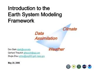
Global modeling and assimilation – Earth System Modeling. 2:00 Intro to Earth System modeling, FIM – Stan Benjamin 2:15 Icosahedral grid in FIM, NIM – Jin Lee 2:30 FIM real-data tests – John Brown

E N D
Global modeling and assimilation – Earth System Modeling 2:00 Intro to Earth System modeling, FIM – Stan Benjamin 2:15 Icosahedral grid in FIM, NIM – Jin Lee 2:30 FIM real-data tests – John Brown 2:40 Global observations for assimilation, NCEP Gridpoint Statistical Interpolation – Dezso Devenyi 2:55 Global assimilation with ensemble Kalman filter – Jeff Whitaker 3:10 Panel discussion – presenters, Andy Jacobson, Georg Grell, Tom Schlatter ESRL Theme Presentation 2:00 – 3:30 PM, Wed 7 May 2008
Offline OR Online An Earth System ModelOr, a Coupled Environmental Model Components Atmosphere – 3d – foundation Include interactive treatment for radiation, clouds (resolved, sub-grid-scale (convective)), turbulent mixing Land-surface/snow/vegetation Usually , e.g., in RUC, WRF, NAM, GFS, etc. Chemistry (AQ, greenhouse gases), aerosols (Carbon Tracker, CMAQ/EPA) (WRF-chem) Ocean, lakes (usually in weather forecast models) Cryosphere – sea ice
An Earth System ModelPrognostic variables Components Atmosphere – 20-100+ levels T, p, u, v, qv, q* (hydrometeors), TKE Land-surface/snow/vegetation – 1-10+ levels T, soil moisture, snow (water equivalent, density, temp) Chemistry (AQ, greenhouse gases), aerosols CO2, CH4, SO2, O3, biogenic/anthropogenic aerosols, 100s more Ocean, lakes (T, p, salinity, …) Cryosphere – (depth, temperature…)
Atmospheric Modeling solutions to partial differential equations for fluid dynamic flowon unevenly heatedrotating sphere Tendency-in-time equations for horizontal wind components, pressure, temperature, moisture variables – e.g., Finite difference representation of atmosphere - cover area to be forecast with 3-d grid of points at which equations will be solved - produce short prediction over short time step (0.5 – 5 min) at each grid point - repeat process until desired forecast length is complete
Earth systems interactions Weather, air quality, climate, biology, agriculture, land surface, oceans, lakes All interact on global to local scales, with various degrees of importance on different scales and for different applications Modified after Carmichael/GURME
Air Quality Modeling: The commonly used approach (“offline”) Weather Forecast model Weather Forecast Weather Data Analysis & Assimilation Snap shots Air quality Forecast model Biogenic and anthropogenic emissions AQ Forecast Chemical, aerosol, removal modules
Air Quality Modeling: The “online” approach Simultaneous forecast of weather and air quality Weather and AQ Forecast Weather Data Analysis & Assimilation & Emissions Chemistry, aerosols, radiation, clouds, temperature, winds Full interaction of meteorology and chemistry (WRF/Chem, applicable to other models)
Global discretization for models Lat-lon representation - GFS, ECMWF, etc Icosahedral grid • Singularities near poles • Requires extra diffusion, longer time steps Nearly equal size of grid volumes, including near poles
NOAA/ESRL Flow-following- finite-volume Icosahedral Model FIM Lat-lon grid - GFS, ECMWF, etc 240km icosahedral grid Level-5 – 10,242 polygons Real-time FIM forecasts- 30km - G8 -655,362
NOAA/ESRL Flow-following- finite-volume Icosahedral Model FIM Jin Lee Sandy MacDonald Rainer Bleck Stan Benjamin Jian-Wen Bao John M. Brown Jacques Middlecoff Ning Wang • Applied in real-data cases down to 15km resolution • MPI implemented with non-structured horizontal grid via ESRL Scalable Modeling System • Scaling efficiency from 120240 procs (98%) • 240480 procs (87%) (for 30km FIM) • Allows variable number of prognostic tracer variables (suitable for air chemistry) +Tom Henderson, Georg Grell, verif/ITS…
FIM design – vertical coordinate • Hybrid (sigma/ isentropic) • vertical coordinate • Adaptive vertical coordinate (θv-σ) • Used in NCEP Rapid Update Cycle (RUC) model (Bleck/Benjamin) • Used in HYCOM ocean model (Bleck) • Option in upcoming WRF repository branch (Zangl – NCAR ) • Improved transport by reducing numerical dispersion from vertical cross-coordinate transport, improved stratospheric/tropospheric exchange. • Applicable down to 1-km non-hydrostatic scale by using larger-scale 3-d isentropic variation as part of FIM target coordinate definition (e.g, Zangl, 2007 - MWR)
8m O3 fcst valid 00z 11 Oct 07 ESRL Global Chemistry/ Atmospheric Model (a work in progress) Current - Georg Grell, Tom Henderson, FIM team Future – Andy Jacobson, others
Asian Dust mid-level Saharan Dust mid-level FIM- with GOCART parameterization (18 aerosols) + GFS physics Dust and Sea-salt, 5-day forecast G5-240km resolution tests here Near-surface sea-salt
Saharan Dust mid-level FIM- with GOCART parameterization (18 aerosols) + GFS physics Dust and Sea-salt, 5-day forecast G7-60km resolution tests here Total PM2.5 (dust and sea-salt, some sulfate) at surface
The bigger picture within NOAA for operational prediction with earth system models- ESMF • Earth System Modeling Framework • Conventions for coupling between earth system model components • Community effort, partially supported by NOAA (also NCAR, NASA, DoD, etc.) • ESMF structure used for NEMS • NOAA Environmental Modeling System • Earth system coupling framework
NEMS Architecture using ESMF Color Key Component class Atmosphere Coupler class unified atmosphere including digital filter Completed Instance Chemistry Under Development WRFchem Future Development Dynamics Physics aerosols Dyn-Phy Coupler ESRL contributions ARW NMM-B NAM Phy Simple FVCORE spectral GFS Phy Regrid, Redist, Chgvar, Avg, etc NOGAPS FIM WRF Phy COAMPS FISL Navy Phy • The goal is one unified atmospheric component that can invoke multiple dynamics and physics. • At this time, dynamics and physics run on the same grid in the same decomposition, so the coupler literally is very simple.
Global Rapid Refresh - hourly updated model at NCEP For aviation, situational awareness 2016- New global satellite ground stations - 40min latency RapidRefresh = RR Global RR = GRR • FIM global model • initial transfer to NCEP – 2010 • candidate for global ensemble w/i ESMF/NEMS • no initial aviation connection • WRF physics, chem options • candidate for Global Rapid Refresh
Global modeling and assimilation – Earth System Modeling 2:00 Intro to Earth System modeling, FIM – Stan Benjamin 2:15 Icosahedral grid in FIM, NIM – Jin Lee 2:30 FIM real-data tests – John Brown 2:40 Global observations for assimilation, NCEP Gridpoint Statistical Interpolation – Dezso Devenyi 2:55 Global assimilation with ensemble Kalman filter – Jeff Whitaker 3:10 Panel discussion – presenters, Andy Jacobson, Georg Grell, Tom Schlatter ESRL Theme Presentation 2:00 – 3:30 PM, Wed 7 May 2008
![Data Modeling [Comparison of data modeling techniques ]](https://cdn0.slideserve.com/205866/data-modeling-comparison-of-data-modeling-techniques-dt.jpg)