Download
1 / 34
340 likes | 463 Views
The Inland Extent of Lake Effect Snow (LES) Bands. Joseph P. Villani NOAA/NWS Albany, NY Michael L. Jurewicz, Sr. NOAA/NWS Binghamton, NY Jason Krekeler NOAA/NWS State College, PA/State University of NY at Albany. Outline. Goals Methodology Results A few case studies/examples Summary.

E N D
The Inland Extent of Lake Effect Snow (LES) Bands Joseph P. Villani NOAA/NWS Albany, NY Michael L. Jurewicz, Sr. NOAA/NWS Binghamton, NY Jason Krekeler NOAA/NWS State College, PA/State University of NY at Albany
Outline • Goals • Methodology • Results • A few case studies/examples • Summary
Goals • Identify atmospheric parameters which commonly have the greatest influence on a LES band’s inland extent • Infuse research findings into operations • Improve forecasts to support NWS Watch/Warning/Advisory program
Satellite depiction of developing LES band Upstream moisture sources Well developed band from Lake Ontario to the Hudson Valley
Methodology/Data Sources • Examined around 25 LES events across the Eastern Great Lakes (Erie/Ontario) during the 2006-2009 time frame • For each event, parameters evaluated at 6-hour intervals (00, 06, 12, and 18 UTC), using mainly 0-hr NAM12 model soundings • Event duration varied from 6 hours to multiple days
Methodology/Data Sources • Wind regimes stratified by mean flows: • 250-290° for single bands (WSW-ENE oriented) • 300-320° for multi bands (NW-SE oriented) • LES bands’ inland extent (miles) calculated from radar mosaics, distance measuring tool • Data points: • Locations inside and north/south band • Data stratified by location relative to band
Example of Data Points Points in and near LES band ALY sounding BUF sounding
Strategy to Determine Best Parameters • Used statistical correlations in Excel spreadsheet to determine most influential factors driving inland extent • Overall, locations relative to bands made little difference in the correlations (within the bands vs. north or south) • A few exceptions
Statistical Correlations • Best correlators to inland extent (all points together): ALY events • 850 hPa Lake-air ∆T (-0.63) • Multi-lake connection present (0.59) • Capping inversion height (0.53) • 0-1 km bulk shear (0.44)
Statistical Correlations • Also notable correlators in locations outside of the bands: • Points south of the band: • Mixed-layer wind speed (0.33) • Mixed-layer directional shear (-0.18) • Points north of the band: • Surface convergence (0.34) • 925 hPa convergence (0.12)
Results from Correlations • Environments that promote greater inland extent: • Multi-Lake Connection • Conditional instability class • Strong 0-1 km shear, weaker shear in1-3 km layer • High capping inversion height
Event Types from Results • Event types favorable for inland extent based on strongest correlations • Instability and Multi-Lake Connection (MLC) • Niziol Instability Class: • Conditional Instability • Lake-850 hPa difference: 12°C to18°C • Lake-700 hPa difference: 17°C to 24°C • Moderate-Extreme Instability • Lake-850 hPa difference: >18°C • Lake-700 hPa difference: >24°C
Classifying Event Types • Use these parameters to classify events: • Type A – MLC & Conditional Instability (most favorable type for inland extent) • Type B – MLC & Moderate/Extreme Instability • Type C – No MLC & Moderate/Extreme Instability • Type D – No MLC & Conditional Instability
Vertical Wind Profiles of Mixed Layer Z 0-3 km 0-1 km X Type A – greater 0-1 km shear, less above 1 km Other Types – less 0-1 km shear, greater above
Type A Sounding - 29Oct2006 18Z Strong 0-1 km speed shear, weaker 1-3 km Little directional shear in mixed layer High (if any) capping inversion Conditional Instability Lake temp: 10°C 850 temp : - 4°C 700 temp: - 15°C 0°C
Upstream Bands Type A – Satellite – 29Oct2006 18Z Broad cyclonic flow associated with Low pressure in Quebec Multi-Lake Connection indicated by visible satellite 850 hPa wind
0-1 km bulk shear Type A – Radar – 29Oct2006 18Z LES band inland extent around 169 mi
Type C Sounding – 07Feb2007 18Z Less 0-1 km speed shear, greater shear in 1-3 km layer More directional shear in mixed layer Extreme Instability Lake temp: 4°C 850 temp : -18°C 700 temp: - 28°C 0°C
No connection with upstream bands Type C – Satellite – 07Feb2007 18Z NO Multi-Lake Connection indicated by visible satellite Well-developed single band, but with little inland extent 850 hPa wind
0-1 km bulk shear Type C – Radar – 07Feb2007 18Z LES band inland extent only 34 mi
Summary • Type A events result in greatest inland extent, often over 100 miles • Key factors are: Instability, MLC, Shear • Ideal conditions: • Conditional instability • MLC • Strong mixed layer flow with minimal speed shear between 1-3 km • Nearly unidirectional flow through mixed layer
Application • Refer to event types when forecasting inland extent • Forecast the event type, which will yield good first guess for inland extent potential • Use pattern recognition of favorable surface, 850/700 hPa low tracks in forecasting MLC • Use AWIPS forecast application (based on equation derived from correlated parameters), which provides estimate of inland extent
Ongoing/Future Work • Infuse forecast applications into operations • Develop graphical interface for output from equation • Evaluate output from AWIPS forecast application
Acknowledgements • Jason Krekeler • NOAA/NWS State College, PA/State University of NY at Albany • Hannah Attard • State University of NY at Albany
References • Niziol, Thomas, 1987: Operational Forecasting of Lake Effect Snowfall in Western and Central New York. Weather and Forecasting. • Niziol, et al., 1995: Winter Weather Forecasting throughout the Eastern United States – Part IV: Lake Effect Snow. Weather and Forecasting.
Questions? Joe.Villani@noaa.gov Michael.Jurewicz@noaa.gov Jason.Krekeler@noaa.gov www.weather.gov/aly www.weather.gov/bgm www.weather.gov/ctp