Download

1 / 13
360 likes | 2.3k Views
Sect. 1.4: D’Alembert’s Principle & Lagrange’s Eqtns. Virtual ( infinitesimal ) displacement Change in the system configuration as result of an arbitrary infinitesimal change of coordinates δ r i , consistent with the forces & constraints imposed on the system at a given time t.

E N D
Sect. 1.4: D’Alembert’s Principle & Lagrange’s Eqtns • Virtual (infinitesimal)displacementChange in the system configuration as result of an arbitrary infinitesimal change of coordinates δri, consistent with the forces & constraints imposed on the system at a given time t. • “Virtual” distinguishes it from an actual displacement dri, occurring in small time interval dt(during which forces & constraints may change)
Consider the system at equilibrium:The total force on each particle is Fi = 0. Virtual work done by Fiin displacement δri: δWi = Fiδri = 0. Sum over i: δW = ∑iFiδri = 0. • Decompose Fiinto applied forceFi(a) & constraint force fi: Fi = Fi(a) + fi δW= ∑i (Fi(a) + fi )δri δW(a)+ δW(c) = 0 • Special case (often true, see text discussion): Systems for which the net virtual work due to constraint forces is zero: ∑ifiδri δW(c) = 0
Principle of Virtual Work Condition for system equilibrium:Virtual work due to APPLIED forces vanishes: δW(a)= ∑iFi(a)δri = 0 (1) Principle of Virtual Work • Note: In general coefficients of δri , Fi(a) 0 even though ∑iFi(a)δri = 0 because δriare not independent, but connected by constraints. • In order to have coefficients of δri = 0, must transform Principle of Virtual Work into a form involving virtual displacements of generalized coordinates q , which are independent. (1) is good since it does not involve constraint forces fi . But so far, only statics. Want to treat dynamics!
D’Alembert’s Principle • Dynamics: Start with Newton’s 2nd Law for particle i: Fi= (dpi/dt) Or: Fi- (dpi/dt) = 0 Can view system particles as in “equilibrium” under a force = actual force + “reversed effective force” = -(dp/dt) • Virtual work done is δW = ∑i[Fi- (dpi/dt)]δri = 0 • Again decompose Fi: Fi = Fi(a) + fi δW= ∑i[Fi(a)- (dpi/dt) + fi]δri = 0 • Again restrict consideration to special case: Systems for which the net virtual work due to constraint forces is zero: ∑i fiδri δW(c) = 0
δW = ∑i[Fi- (dpi/dt)]δri = 0 (2) D’Alembert’s Principle • Dropped the superscript (a)! • Transform (2) to an expression involving virtual displacements of q(which, for holonomic constraints, are indep of each other). Then, by linear independence, the coefficients of the δq= 0
δW = ∑i[Fi- (dpi/dt)]δri = 0(2) • Much manipulation follows! Only highlights here! • Transformation eqtns: ri = ri(q1,q2,q3,.,t) (i = 1,2,3,…n) • Chain rule of differentiation (velocities): vi (dri/dt) = ∑k(ri/qk)(dqk/dt) + (ri/t) (a) • Virtual displacements δriare connected to virtual displacements δq: δri= ∑j (ri/qj)δqj(b)
Generalized Forces • 1st term of (2)(Combined with (b)): ∑i Fiδri = ∑i,j Fi(ri/qj)δqj ∑jQjδqj (c) Define Generalized Force (corresponding to Generalized Coordinate qj): Qj ∑iFi(ri/qj) • Generalized Coordinates qj need not have units of length! Corresponding Generalized ForcesQj need not have units of force! • For example: If qj is an angle, corresponding Qj will be a torque!
2nd term of (2) (using (b) again): ∑i(dpi/dt)δri = ∑i[mi(d2ri/dt2)δri ] = ∑i,j[mi(d2ri/dt2)(ri/qj)δqj](d) • Manipulate with (d):∑i[mi(d2ri/dt2)(ri/qj)] = ∑i[d{mi(dri/dt)(ri/qj)}/dt] – ∑i[mi(dri/dt)d{(ri/qj)}/dt] Also: d{(ri/qj)}/dt = {dri/dt}/qj (vi/qj) Use (a):(vi/qj) = ∑k(2ri/qjqk)(dqk/dt) + (2ri/qjt) From (a):(vi/qj) = (ri/qj) So: ∑i[mi(d2ri/dt2)(ri/qj)] = ∑i[d{mivi(vi/qj)}/dt] - ∑i[mivi(vi/qj)]
More manipulation (2) is: ∑i[Fi-(dpi/dt)]δri = 0 ∑j{d[(∑i (½)mi(vi)2)/qj]/dt - (∑i(½)mi(vi)2)/qj - Qj}δqj= 0 • System kinetic energy is: T (½)∑imi(vi)2 D’Alembert’s Principle becomes ∑j{(d[T/qj]/dt) - (T/qj) - Qj}δqj= 0 (3) • Note: If qjare Cartesian coords, (T/qj) = 0 In generalized coords, (T/qj) comes from the curvature of the qj. (Example: Polar coords, (T/θ) becomes the centripetal acceleration). • So far, no restriction on constraints except that they do no work under virtual displacement. qj are any set. Special case:Holonomic Constraints It’s possible to find sets of qj for which each δqjis independent. Each term in (3) is separately 0!
Holonomic constraints D’Alembert’s Principle: (d[T/qj]/dt) - (T/qj) = Qj (4) (j = 1,2,3, … n) • Special case: A Potential ExistsFi= - iV • Needn’t be conservative! V could be a function of t! Generalized forces have the form Qj ∑i Fi(ri/qj) = - ∑i iV(ri/qj) - (V/qj) • Put this in (4):(d[T/qj]/dt) - ([T-V]/qj) = 0 • So far, V doesn’t depend on the velocities qj (d/dt)[(T-V)/qj] - (T-V)/qj = 0 (4´)
Lagrange’s Equations • Define:The LagrangianL of the system: L T - V Can write D’Alembert’s Principle as: (d/dt)[(L/qj)] - (L/qj) = 0 (5)(j = 1,2,3, … n) (5) Lagrange’s Equations
Lagrange’s Eqtns • Lagrangian:L T - V • Lagrange’s Eqtns: (d/dt)[(L/qj)] - (L/qj) = 0 (j = 1,2,3, … n) • Note:L is not unique, but is arbitrary to within the addition of a derivative (dF/dt). F = F(q,t) is any differentiable function of q’s & t. • That is, if we define a new Lagrangian L´ L´= L + (dF/dt) It is easy to show that L´satisfies the same Lagrange’s Eqtns (above).