Download
1 / 81
810 likes | 828 Views
This lecture covers the Simple Protocol, Stop-and-Wait Protocol, Go-Back-N Protocol, and Selective-Repeat Protocol in Chapters 13 and 16 of the textbook. It also discusses the Stream Control Transmission Protocol (SCTP) and FSMs for these protocols.

E N D
(1) Transport Layer Protocols • Simple Protocol • Stop-and-Wait Protocol • Go-Back-N Protocol • Selective-Repeat Protocol • Bidirectional Protocols: Piggybacking (2) SCTP – Stream Control Transmission Lecture
Simple protocol • Simple Protocol has no Error Control or Flow Control • The both the Tx and Rx are always in the “Ready” state • Tx can’t send a message until the Sending Application layer has a message to send • When the message is ready to be sent, it is then encapsulated in a packet and sent to the Rx • The Rx is in the “Ready” state until it receives a packet from the Tx, then Rx decapsulates the message out of the packet and send it to the receiving process. FSMs for simple protocol Lecture
Stop-and-wait Protocol • Stop-and-Wait Protocol is a connection-oriented protocol with Error Control and Flow Control • Both the Tx and Rx uses a sliding window of size 1 • Tx sends one packet at a time and waits for an acknowledgement • A checksum is used in the packet for the Rx to detect errors. • Tx uses a timer every time it sends a packet • If Tx receives an ACK before the timer counts down, it sends the NEXT packet • If Tx doesn’t receive an ACK before the timer counts down, it resends the previous packet • If Tx doesn’t receive an ACK before the timer counts down because the ACK itself is lost or corrupted, the Tx will resend the previous packet – creating a duplicate at the Rx side – the Rx will know it has duplicates because both packets will have the SAME sequence number • Therefore, the Tx holds the packets until it receives an ACK • If Rx detects an error, the packet is dropped and no acknowledgment is sent • FLOW CONTROL is achieved by Tx waiting for an ACK before sending • ERROR CONTROL is achieved by the Rx dropping bad packets and allowing the Tx to re-send Lecture
FSMs for stop-and-wait protocol If time out event occurs, resend packet and remain in blocking state If corrupted ACK received or ACK not related to packet, drop ACK and remain in blocking state until time-out occurs –then resend packet Send packet, go into blocking state While in blocking state, if error-free ACK received, go to ready state If good packet received with the expected sequence number, send an ACK about the packet and remain in the ready state expecting the next packet If corrupted packet received, drop it and remain in ready state If good packet received without the expected sequence number, drop the packet because it is a duplicate, send an ACK about the packet and remain in the ready state expecting the next packet Lecture
Stop-and-wait Protocol Example (2) Packet0 arrives and ACK pointing to the next packet is sent back (1) Packet created with Seq# 0 and sent and time starts (3) ACK comes back and match next Seq#, so sent packet is removed out of storage (5) Packet lost and doesn’t arrive before time out (4) Packet created with with next Seq# 1 and sent and time starts (7) Packet1 arrives and ACK pointing to the next packet is sent back (6) Try resending packet 1 (8) ACK comes back and match next Seq#, so sent packet is removed out of storage (10) Packet0 arrives and ACK pointing to the next packet is sent back but lost enroute (9) Packet created with with next Seq# 0 and sent and time starts (11) ACK not received in time, so Packet0 is resent (12) Packet0 arrives AGAIN, so duplicate occurs because Rx was expecting packet1 (and not packet0) (13) ACK comes back and match next Seq#, so sent packet is removed out of storage Lecture
Stop-and-wait Protocol Bandwidth-Delay-Product • The data-rate (or bandwidth) TIMES the length of the pipe (or round-trip delay), tells the volume of the pipe in bits • A small pipe with a low data rate with have LESS VOLUME of bits than a large/fat pipe with a high data rate • For Stop-and-wait, not many bits are being sent at once because it is done sequentially – therefore, the stop-and-wait protocol is inefficient when it comes to the bandwidth-delay-product Pipelining • Pipelining is starting new tasks before the previous task (or tasks) is completed • Pipelining improves the efficiency of transmission by increasing the number of bits in transition with respect to the bandwidth-delay-product • Stop-and-wait protocol doesn’t use pipelining because the previous task must be acknowledged before the next starts Lecture
Go-Back-N protocol • Go-Back-N protocol improves efficiency (filling of the pipe) by allowing multiple packets to be in transition while the Tx is waiting for acknowledgments • Several packets can be sent before the Tx receives an ACK, however the Rx can only buffer one packet at a time • Tx keeps copies of the sent packets until ACK is received • Sequence number is modulo 2m , where m is the number of bits in the sequence number field • The ACK number is cumulative – it keeps track of the next packet expected – if ACK#=4, that means all packets up to 3 have arrive successfully Lecture
Go-Back-N protocol • Sf is the first outstanding packet to be sent that has not been ACK • Sn is the next packet to be sent • Ssize is the send window size • Rn is the sequence number of the next packet to be received at the Rx • Tx keeps copies of the sent packets until ACK is received SENT Window - Four possible cases for sequence number The send window can slide one or more slots when an error-free ACK with ackNo between Sf and Sn arrives. Sequence numbers that can’t be used until the window slides Lecture
Sliding the Go-Back-N send window Receive window for Go-Back-N • The Rx is always looking for the arrival of a specific packet –all other packets received are discarded • A timer is only used for the FIRST outstanding packet (packets that have not been ACK) • If the timer expires, ALL outstanding packets must be resent • Suppose the Tx has already sent packet 5, so the next packet to be sent is 6 (Sn=6) – and lets say packet 2 was the initial outstanding packet to be sent (Sn=2) – if the timer expired, packets 2, 3, 4, and 5 will all have to be resent – this is the reason this protocol is called Go-Back-N Lecture
Go-Back-N protocol Example Initialization Packet0 sent and ACK1 comes back So packet0 is moved from storage Packet1 is sent and ACK2 is lost – in the meanwhile, packet2 and packet3 are sent ACK3 comes back before ACK2, because ACK2 was lost Because the ACK are cumulative, ACK3 coming back means both packets 1 and 2 were successfully received – so packets 1 and 2 are moved from storage Lecture
Selective-Repeat Protocol • Go-Back-N simplifies the process at the Rx however, it is inefficient because if one packet is out-of-order or corrupted, it could resend other packets that are NOT corrupted. This protocol could cause traffic to increase greatly, causing the network to collapse. • Selective-Repeat Protocol only resends the individual packets that are corrupted or lost. • For Selective-Repeat, the receiver window is larger than 1 and is the same size as the Tx window Lecture
Send window for Selective-Repeat protocol Receive window for Selective-Repeat protocol • The ACK sent from the Rx is for each individual packet successfully received Lecture
Selective-Repeat Protocol Example Not pointing to next packet – but rather current packet received Lecture
Design of piggybacking for Go-Back-N • The protocols thus far were all presented as being “unidirectional” – data packets flow in only one direction (from Tx to Rx) – and ACK packets flow in only one direction (Rx to Tx) • In real life for client-server, data packets flow in both directions – therefore, ACK packets need to flow in both directions. • Piggypacking is when the data packets also carry the ACK • For example, when a packet is carrying data from Tx to Rx, it can also carry an ACK about a data packet sent from the Rx to Tx • Piggybacking improves efficiency of the bidirectional protocols Lecture
OBJECTIVES: • To introduce SCTP as a new transport-layer protocol. • To discuss SCTP services and compare them with TCP. Outline • 16.1 Introduction • 16.2 SCTP Services • 16.3 SCTP Features Lecture
SCTP - INTRODUCTION Stream Control Transmission Protocol (SCTP) is a new reliable, message-oriented transport-layer protocol. SCTP lies between the application layer and the network layer and serves between the application programs and the network operations. SCTP is designed for recently introduced Internet apps like ISDN-over-IP, telephony signaling, media gateway control, and IP telephony SCTP provides more enhanced performance and reliability than TCP. Lecture
SCTP - INTRODUCTION • UDP is a “message-oriented” protocol because UDP encapsulates the message into the datagram and sent over the network – each message is independent from any other message – this is a desirable feature for “real-time data” type apps – the problem with UDP is, it is unreliable and packets can be lost and it doesn’t have flow or congestion control • TCPis a “byte-oriented” protocol because it receives a message (or messages) and stores them as a stream of bytes and sends them in segments. TCP doesn’t preserve the message boundaries. However, TCP is reliable with congestion and flow control - it can detect duplicates, lost packets are resent and bytes are delivered in order. • SCTP combines the best features from UDP and TCP with some additional features – it preserves the message boundaries and able to detect duplicates, resend lost packets and deliver packets in order. It also has congestion and flow control mechanisms. Lecture
SCTP Services provided to Application Layer Processes • Process-to-Process Communication • Multiple Streams • Multihoming • Full-Duplex Communication • Connection-Oriented Service • Reliable Service Process-to-Process Communications • SCTP uses well-known ports Lecture
Multiple-stream concept • TCPuses streams – each connection between a client and server involves streams being sent – the problem is, if there is a lost, multiple data is lost – not acceptable for real-time data type apps. • SCTP allows multiple streams for a connection at the same time – so if one stream has a problem and is blocked, some other stream will get the data to the process – this is called “association” in SCTP terminology. Lecture
Multihoming concept • A TCPconnection involves only two IP addresses – one for the Tx and another for the Rx • In implementing an “SCTP association” or “multiple streams”, multiple connections must be made – therefore both the Tx and Rx must multiple IP addresses on both ends – this is called “multihoming” • Typically SCTP will have a single “main” connection and an “alternative” connection if the main connection fails • SCTP does not use the multiple connections for “load sharing” between Tx and Rx Server connected to two local networks with two IP addresses Client connected to two local networks with two IP addresses Lecture
More SCTP Services provided to Application Layer Processes • FULL-DUPLEX COMMUNICATION - data can flow in both directions – therefore buffers are used at both ends • CONNECTION-ORIENTED SERVICE– like TCP, SCTP establishes a relationship upfront before the sending and receiving occurs – the only difference is, SCTP establishes an “association” upfront. • RELIABLE SERVICE – like TCP, SCTP uses ACK for error control Lecture
SCTP Features • NOTE:For SCTP, a stream could consists of multiple sequences of messages (or multiple ordered sets of messages). For TCP, a segment consisted of a “sequence of bytes” and a message could have multiple segments • TRANSMISSION SEQUENCE NUMBER (TSN) - The unit of data for TCP is the byte and recall that TCP numbers bytes using the sequence numbers. SCTP’s unit of data is the “chunk” and may or may not have a one-to-one relationship with the “message” due to fragmentation. If a message is very large, it could consists of multiple chunks. SCTP uses a transmission-sequence-number in numbering data chunks. TSNs are 32 bits and are randomly initialized. Each chunk carries a TSN in its header. • STREAM IDENTIFIER (SI)– for TCP, there is only one stream. For SCTP, there could be multiple streams. Each stream is identified by a stream identifier (SI) – the SI is also in the chuck’s header. The SI is 16 bits starting from 0. Think of this “stream” as the connection or path. • STREAM SEQUENCE NUMBER (SSN) – there could be multiple “chunks” associated with a message and multiple messages associated with a stream. Each data chunks uses the stream sequence number to associate with the appropriate stream (or group of messages) on the Rx side. SSN use tp distinguish between different data chunks belonging to the same stream. Think of this “stream” as a collection of chunks belonging to the same group at the Rx side. Lecture
SCTP Features continue • FLOW CONTROL - Like TCP, SCTP implements flow control • ERROR CONTROL– Like TCP, SCTP implements error control. • CONGESTION CONTROL – Like TCP, SCTP implements congestion control to determine how many data chunks can be injected into the network. Lecture
Comparison between a TCP segment and an SCTP packet • In TCP, a user datagram carried both data and control information – the form of bytes • SCTP is different – data is carried in chunks and control info is carried in chunks • For SCTP, several data and control chunks can be packaged in a packet • A “packet” for SCTP is the same as a “segment or user-datagram” for TCP Lecture
TCP segment Versus SCTP packet • For TCP, control info is in the header; For SCTP, control info is in a chuck – and there can be different types of control chunks • For TCP, the datagram is treated as one entity; For SCTP, the packet can carry several chunks – and each chunk can belong to a different stream • For TCP, options can be a part of the segment; For SCTP, options are in chunks – and new option chunks can be defined • TCP minimum header size is 20 bytes; SCTP header is 12 bytes – some of the info is located in other chunks • TCP checksum is 16 bits; SCTP checksum is 32 bits • TCP uses socket addresses; SCTP uses the “verification tag” to id the “association” • TCP uses the sequence number; SCTP uses the TSN, IS and SSN Lecture
SCTP Packets, Data chunks, and Streams • An association may send many packets • A packet may contain several chunks • Chunks may belong to different streams • If a message is very long, it can be carried by several chunks. • But typically, a message can fit into a single chunk Lecture
Packet, data chunks, and streams • In better understanding this, lets assume an application process delivers 11 messages to SCTP, where each message is earmarked for an appropriate stream • It delivers all messages belonging to the first stream first, then all messages belonging to the second stream second, and finally, all messages belonging to the last stream last. (keep in mind it could have been mixed). • If the network can only handle 3 data chunks per packet, we will need 4 packets (because 11/3 = 3.66 = 4) • Data chunks for stream 0 are carried in the 1st and 2nd packet; data chunks for stream 1 are carried in the 2nd and 3rd packet; data chunks for stream 2 are carried in the 3rd and 4th packets • TSN is a cumulative number and used for flow and error control; SI defines the stream to which the chunk belongs; SSN defines the chunk’s order in a particular stream (SSN starts from 0 for each stream) Lecture
SCTP Acknowledgments • TCP’s acknowledgment number is byte-oriented • SCTP’s acknowledgment number is chunk-oriented Lecture
Also called , IPng – “IP next generation” Next Generation: IPv6 and ICMPv6 Recall IPv4 provides host-to-host or hop-to-hop communication Recall UDP/TCP provide end-to-end or process-to-process communication
Why IPv6 ? 3 major reasons Recall that (1) subnetting, (2) classless addressing, (3) DHCP (dynamic address allocation) and (4) NAT all contributed to better utilization of the 32-bit address space - despite these solutions, address depletion is still an issue There are numerous applications on the rise that require streaming real-time audio and video – and real-time transmission requires minimum delay and reservation-of-resources strategies – and IPv4 isn’t designed for these strategies Over the last few years, there has been a much greater demand for security and for the Internet to accommodate encryption and authentication of data for some applications – and IPv4 doesn’t provide encryption or authentication
Why IPv6 ? IPv6 was proposed in overcoming IPv4’s deficiencies IPv6 has these advantages over IPv4: 1. larger address space – 128 bits 2. better header format – options can be inserted or not 3. new options – additional functionalities4. allowance for extension – protocol can be extended for newer technologies5. support for resource allocation – enables the Tx to request special handling 6. support for more security – provides encryption and authentication Related protocols were either modified or dropped for IPv6 - ICMP was modified (ICMPv6) - ARP and IGMP in version 4 were combined in ICMPv6 - RARP was dropped - RIP and OSPF were slightly modified
IPv6 Address Uses hexadecimal colon notation, a 296 address increase over IPv4 Abbreviated address Leading zeros can be omitted If consecutive sections consist of zeros only, the zeros can be removed altogether and replaced with double semicolon Only allowed once per address – if there were two runs of zero sections, only one can be abbreviated
IPv6 Address Like IPv4, IPv6 can use CIDR notation 3 Categories of IPv6 Addresses Unicast Address – packet sent to a specific computer Anycast Address – group of computers with addresses that have the same prefix (ie. all belong to the same physical network) Multicast Address – packet sent to a group of computers with different address prefixes
IPv6 Address Address structure Means 1/8 of the entire address spaces uses type prefix 010 The address space has many purposes The address space is divided into 2 parts The first part, called “type prefix”, is variable length, defines the purpose by using unique codes Type prefixes for IPv6 addresses
IPv6 Address Type prefix 010 or provider-based address is generally used by a host as a unicast address Provider-based address structure Variable-length field identifies the provider for Internet access (ie ISP) – recommends this field be 16 bits The provider (ISP) assigns a 24-bit subscriber id to the organization Identifies one of many subnets under the subscriber’s control – recommends using 32-bits Identifies the node connected to the subnet – recommends 48-bits (the same as the 48-bit physical Ethernet address) Defines the address as a provider-based address Indicates one of the three agencies that has registered the address. INTERNIC – North America RIPNIC – Europe APNIC – Asia & Pacific
IPv6 Address Can think of the provider-based address as a hierarchical identity with several prefixes Address hierarchy
IPv6 Address Unspecified address When the non-prefix part of the address is also zeros – this is called an Unspecified Address – this address is used when the host doesn’t know its own address and sends an inquiry and uses the Unspecified Address to represent itself – the address can not be used as a destination address Loopback address Recall the purpose of the loopback address – an address used by a host to test itself without going into the network.
IPv6 Address During transition from IPv4 to IPv6, hosts can use their IPv4 addresses embedded in IPv6 addresses. Two formats have been designed for this – (1) compatible and (2) mapped Compatible address 96 bits of zeros followed by 32 bits of IPv4 address Compatible Address is used when a IPv6 Tx wants to send a message to an IPv6 Rx, but needs to pass through a region using IPv4 – the Tx must them use the compatible address while passing through the Ipv4 region 0000 0010 0001 0001 0000 1101 0000 1110 Binary 02 0D 11 0E Hexidecimal Decimal 2 13 17 14
IPv6 Address During transition from IPv4 to IPv6, hosts can use their IPv4 addresses embedded in IPv6 addresses. Two formats have been designed for this – (1) compatible and (2) mapped Mapped address 80 bits of zeros followed by 16 bits of ones followed by 32 bits of IPv4 address Mapped Address is used when a IPv6 Tx wants to send a message to an IPv4 Rx. The packet will mostly travel through an IPv6 region with a final destination of IPv4. NOTE: when calculating the CHECKSUM, either the embedded address or total address can be used because the extra 0s or 1s (in multiples of 16) DO NOT have an effect on the checksum calculation.
IPv6 Address Addresses that use the reserved prefix (11111110) are local addresses Link local address Used if the LAN uses the Internet protocols but is not connected to the Internet for security reasons – these addresses do not have a global effect Site local address Used if a site with several networks uses the Internet protocols but is not connected to the Internet for security reasons – these addresses do not have a global effect
IPv6 Address Addresses used to define a group of hosts instead of just one. Multicast address Defines the group address as either permanent or transient Permanent Address – defined by the Internet authorities and can be accessed at all time Transient Address – is temporary Defines the scope of the group address
Next Generation: IPv6 and ICMPv6 .. Continuing …
Format of an IPv6 datagram Defines the priority of the packet with respect to traffic congestion (discuss later) 24-bit field that provide special handling for a particular flow of data (discuss later) Defines the version (IPv6 = 6) 8-bit field defining the header that follows the base header (discuss later) 8-bit field serves as the Time-To-Live (TTL) 2-byte field defines the length of the data excluding the base header Source address Usually identifies the destination address – if Source Routing is used, identifies the address of the next router
Format of an IPv6 datagram Next Header The next header is either one of the optional extension headers used by IPv6 or the header of an encapsulated packet such as UDP or TCP. Each extension header also contains the next header field. For version 4, this field was called the protocol. Next header codes
Format of an IPv6 datagram Priority Defines the priority of each packet with respect to other packets from the same source. IPv6 divides traffic into two categories: congestion-control and non-congestion-control Priorities for congestion-controlled traffic Process does not define a priority If a source adapts itself to traffic slowdown when there is congestion, the traffic is called congestion-control traffic – example, TCP sliding window protocol Defines data delivered in the background User is not waiting for the data (ie. Email) Protocol that transfer data while the user is waiting to receive the data (ie FTP, HTTP) User interaction is needed (ie. TELNET) Protocols that control traffic (ie. OSPF, RIP, SNMP)
Format of an IPv6 datagram Priority Defines the priority of each packet with respect to other packets from the same source. IPv6 divides traffic into two categories: congestion-control and non-congestion-control Priorities for non congestion-controlled traffic Refers to traffic that expects minimum delay – dropping packets is not desired – retransmission is impossible. Examples would be realtime audio and video
IPv6 Packet Flow Label • Recall how a routing-algorithm table lookup is performed for a packet using a router. • Sequence of packets sent from a Tx to Rx needing “special handling” is called a flow • Combo of the Tx address and a flow label uniquely identifies a flow of packets • The flow label is assigned to the packet by the Tx – randomly generated number • From a router perspective, a flow is a sequence of packets sharing the characteristics (using same resources, same security, , etc) • If the packet has a flow number, the router consults it flow label table for the next hop • This speeds up the process – much faster than going through the routing algorithm approach • Flow label approach is good for apps needing to reserve bandwidth and buffer space beforehand in minimizing delays (ie. realtime audio and video)