Statistical Properties of Wave Chaotic Scattering and Impedance Matrices

1. Statistical Properties of Wave Chaotic Scattering and Impedance Matrices Collaborators: Xing Zheng, Ed Ott, Experiments Sameer Hemmady, Steve Anlage, Supported by AFOSR-MURI

2. Schematic • Coupling of external radiation to computer circuits is a complex processes: apertures resonant cavities transmission lines circuit elements • Intermediate frequency range involves many interacting resonances • System size >>Wavelength • Chaotic Ray Trajectories Integrated circuits cables connectors circuit boards • What can be said about coupling without solving in detail the complicated EM problem ? • Statistical Description ! (Statistical Electromagnetics, Holland and St. John) Electromagnetic Coupling in Computer Circuits

3. N- Port System N ports • voltages and currents, • incoming and outgoing waves • • • S matrix Z matrix Z(w) , S(w) • Complicated function of frequency • Details depend sensitively on unknown parameters voltage current outgoing incoming Z and S-MatricesWhat is Sij ?

4. Mean spacing df ≈ .016 GHz Lossless: Zcav=jXcav  S - reflection coefficient Zcav Frequency Dependence of Reactance for a Single Realization

5. S 1 2 S Reciprocal: Transmission Lossless: Reflection = 1 - Transmission Two - Port Scattering Matrix

6. Port 1 Losses Statistical Model Impedance Other ports RR1(w) Port 2 Radiation Resistance RRi(w) System parameters RR2(w) Dw2n - mean spectral spacing Port 1 Q -quality factor Free-space radiation Resistance RR(w) ZR(w) = RR(w)+jXR (w) wn - random spectrum Statistical parameters win- Guassian Random variables Statistical Model of Z Matrix

7. ports h Box with metallic walls Only transverse magnetic (TM) propagate for f < c/2h Ez Hy Hx Voltage on top plate • Anlage Experiments • Power plane of microcircuit Two Dimensional Resonators

8. • Cavity fields driven by currents at ports, (assume ejwt dependence) : k=w/c Profile of excitation current • Voltage at jth port: • Impedance matrix Zij(k): • Scattering matrix: Wave Equation for 2D Cavity Ez =-VT/h

9. Preprint available: Five Different Methods of Solution Problem, find: 1. Computational EM - HFSS 2. Experiment - Anlage, Hemmady 3. Random Matrix Theory - replace wave equation with a matrix with random elements No losses 4. Random Coupling Model - expand in Chaotic Eigenfunctions 5. Geometric Optics - Superposition of contributions from different ray paths Not done yet

10. Where: 1. fn are eigenfunctions of closed cavity 2. kn2 are corresponding eigenvalues Expand VT in Eigenfunctions of Closed Cavity Zij - Formally exact

11. 1. Replace eigenfunction with superposition of random plane waves Random amplitude Random direction Random phase Random Coupling ModelReplace fn by Chaotic Eigenfunctions

12. Time reversal symmetry is a Gaussian random variable Time reversal symmetry broken kj uniformly distributed on a circle |kj|=kn Chaotic Eigenfunctions

13. Chaotic Integrable (not chaotic) Mixed Chaotic Cavity Shapes

14. Eigenfrequency Statistics 2. Eigenvalues kn2 are distributed according to appropriate statistics Mean Spacing: 2D 3D Normalized Spacing:

15. Thorium 2+O TRSB TRS Poisson Harmonic Oscillator energy Wave Chaotic Spectra Spacing distributions are characteristic for many systems TRS = Time reversal symmetry TRSB = Time reversal symmetry broken

16. Statistical parameters win- Guassian Random variables kn - random spectrum Statistical Model for Impedance Matrix System parameters -Radiation resistance for port i Dk2n=1/(4A) - mean spectral spacing Q -quality factor

17. • Mean and fluctuating parts: • Mean part: (no losses) Radiation reactance • Fluctuating part: Lorenzian distribution -width radiation resistance RRi Predicted Properties of Zij

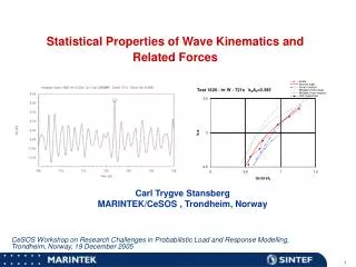
18. Curved walls guarantee all ray trajectories are chaotic Moveable conducting disk - .6 cm diameter “Proverbial soda can” HFSS - SolutionsBow-Tie Cavity Cavity impedance calculated for 100 locations of disk 4000 frequencies 6.75 GHz to 8.75 GHz

19. Frequency Dependence of Reactance for a Single Realization Mean spacing df ≈ .016 GHz  Zcav=jXcav

20. Frequency Dependence of Median Cavity Reactance Df = .3 GHz, L= 100 cm Median Impedance for 100 locations of disc  Effect of strong Reflections ? Radiation Reactance HFSS with perfectly absorbing Boundary conditions

21. Distribution of Fluctuating Cavity Impedance 6.75-7.25 GHz 7.25-7.75 GHz Rfs ≈ 35  x x 7.75-8.25 GHz 8.25-8.75 GHz x x

22. Port Lossless 2-Port Z’cav(w) = j(X’R(w)+x R’R(w)) Cavity Impedance: Zcav(w) Zcav(w) = j(XR(w)+x RR(w)) Unit Lorenzian Unit Lorenzian Port Free-space radiation Impedance ZR(w) = RR(w)+jXR(w) Lossless 2-Port Impedance Transformation by Lossless Two-Port Z’R(w) = R’R(w)+jX’R(w)

23. Eigenvalues of Z matrix q2 Individually x1,2 are Lorenzian distributed Distributions same as In Random Matrix theory q1 Properties of Lossless Two-Port Impedance

24. HFSS Solution for Lossless 2-Port Joint Pdf for q1 andq2 Disc q2 Port #1: (14, 7) Port #2: (27, 13.5) q1

25. Port 1 Losses Other ports Zcav = jXR+(r+jx) RR Distribution of reactance fluctuations P(x) Distribution of resistance fluctuations P(r) Effect of Losses

26. Predicted and Computed Impedance Histograms Zcav = jXR+(r+jx) RR

27. Equivalence of Losses and ChannelsZcav = jXR+(r+jx) RR Distribution of resistance fluctuations P(r) Distribution of reactance fluctuations P(x) x r r x

28. Role of Scars? • Eigenfunctions that do not satisfy random plane wave assumption • Scars are not treated by either random matrix or chaotic eigenfunction theory • Semi-classical methods Bow-Tie with diamond scar

29. 47.4 cm Large Contribution from Periodic Ray Paths ? 22 cm 11 cm Possible strong reflections L = 94.8 cm, Df =.3GHz