Heuristic Search
Heuristic Search. Jacques Robin. Outline. Definition and motivation Taxonomy of heuristic search algorithms Global heuristic search algorithms Greedy best-first search A* RBFS SMA* Designing heuristic functions Local heuristic search algorithms Hill-climbing and its variations

Heuristic Search
E N D
Presentation Transcript
Heuristic Search Jacques Robin
Outline • Definition and motivation • Taxonomy of heuristic search algorithms • Global heuristic search algorithms • Greedy best-first search • A* • RBFS • SMA* • Designing heuristic functions • Local heuristic search algorithms • Hill-climbing and its variations • Simulated annealing • Beam search • Limitations and extensions • Local heuristic search in continuous spaces • Local heuristic online search • Local heuristic search for exploration problems
Heuristic Search:Definition and Motivation • Definition: • Non-exhaustive, partial state space search strategy, • based on approximate heuristic knowledge of the search problem class (ex, n-queens, Romania touring) or family (ex, unordered finite domain constraint solving) • allowing to leave unexplored (prune) the state space from zones that are either guaranteed orunlikely to contain a goal state (or a utility maximizing state or cost minimizing path) • Note: • An algorithm that uses a frontier node orderingheuristic to generate a goal state faster, • but is still ready to generate all state space states if necessary to find goal state • i.e., an algorithm that does no pruning • is not a heuristic search algorithm • Motivation: exhaustive search algorithms do not scale up, • neither theoretically (exponential worst case time or space complexity) • nor empirically (experimentally measured average case time or space complexity) • Heuristic search algorithms do scale up to very large problem instances, in some cases by giving up completeness and/or optimality • New data structure: heuristic function h(s)estimates the cost of the path from a fringe state s n to a goal state
Best-First Global Search • Keep all expanded states on the fringe • just as exhaustive breadth-first search and uniform-cost search • Define an evaluation function f(s) that maps each state onto a number • Expand the fringe in order of decreasing f(s) values • Variations: • Greedy Global Search (also called Greedy Best-First Search) defines f(s) = h(s) • A* defines f(s) = g(s) + h(s) • where g(s) is the real cost from the initial state to the state s, • i.e., the value used to choose the state to expand in uniform cost search
Greedy Local Search Characteristics • Strengths: simple • Weaknesses: • Not optimal • because it relies only on estimated cost from current state to goal • while ignoring confirmed cost from initial state to current state • ex, misses better path through Riminicu and Pitesti • Incomplete • can enter in loop between two states that seem heuristically closer to the goal but are in fact farther away • ex, from Iasi to Fagaras, it oscillates indefinitely between Iasi and Meant because the only road from either one to Fagaras goes through Valsui which in straight line is farther away to Fagaras than both
h(s): straight-line distance to Bucharest: 75 + 374 239 239 + 178 220 140 + 253 118 + 329 220 + 193 317 317 + 98 418 366 455 336 + 160 A* Example 449 417 393 447 413 415 496
A* Search Characteristics • Strengths: • Graph A* search is complete and Tree A* search is complete and optimal if h(s) is an admissible heuristic, i.e., if it never overestimates the real cost to a goal • Graph A* search if optimal if h(s) admissible and in addition a monotonic (or consistent) heuristic • h(s) is monotonic iff it satisfies the triangle inequality, i.e.,s,s’ stateSpace (a actions, s’ = result(a,s)) h(s) cost(a) + h(s´) • A* is optimally efficient,i.e., no other optimal algorithm will expand fewer nodes than A* using the same heuristic function h(s) • Weakness: • Runs out of memory for large problem instance because it keeps all generated nodes in memory • Why? • Worst-case space complexity = O(bd), • Unless n, |h(n) – c*(n)| O(log c*(n)) • But very few practical heuristics verify this property
A* Search Characteristics • A* explores generates a contour around the best path • The better the heuristic estimates the real cost, the narrower the contour • Extreme cases: • Perfect estimates, A* only generates nodes on the best path • Useless estimates, A* generate all the nodes in the worst-case, i.e., degenerates into uniform-cost search
Recursive Best-First Search (RBFS) • Fringe limited to siblings of nodes along the path from the root to the current node • For high branching factors, this is far smaller than A*’s fringe which keeps all generated nodes • At each step: • Expand node n with lowest f(n) to generate successor(n) = {n1, ..., ni} • Store at n: • A pointer to node n’ with the second lowest f(n’) on the previous fringe • Its cost estimate f(n’) • Whenever f(n’) f(nm) where f(nm) = min{f(n1), ..., f(ni)}: • Update f(n) with f(nm) • Backtrack to f(n’)
RBFS: Characteristics • Complete and optimal for admissible heuristics • Space complexity O(bd) • Time complexity hard to characterize • In hard problem instance, • can loose a lot of time swinging from one side of the tree to the other, • regenerating over and over node that it had erased in the previous swing to that direction • in such cases A* is faster
Heuristic Function Design • Desirable properties: • Monotonic, • Admissible, i.e.,s stateSpace, h(s) c*(s), where c*(s) is the real cost of s • High precision, i.e., as close as possible to c* • Precision measure: effective branching factor b*(h) 1, • N = average number of nodes generated by A* over a sample set of runs using h has heuristic • Obtained by solving the equation: b*(h) + (b*(h))2 + ... + (b*(h))d = N • The closer b*(h) gets to 1, the more precise h is • h2 dominates h1 iff: s stateSpace, h1(s) h2(s),i.e., if b*(h1) closer to 1 than b*(h2) • hd(n) = max{h1(n), .., hk(n)} always dominates h1(n), .., hk(n) • General heuristic function design principle: • Estimated cost = actual cost of simplified problem • computed using exhaustive search as a cheap pre-processing stage • Problem can be simplified by: • Constraint relaxation on its actions and/or goal state, which guarantees admissibility and monotonicity • Decomposition in independent sub-problems
Constraints: Tile cannot move diagonally Tile cannot move in occupied location Tile cannot move directly to non-neighboring locations Relaxed problem 1: Ignore all constraints h1: number of tiles out of place Relaxed problem 2: Ignore only constraint 2 h2: sum over all tiles t of the Manhattan distance between t’s current and goal positions h2 dominates h1 Heuristic Function Design: Constraint Relaxation Example
Preprocessing for one problem class amortized over many run of different instances of this class For each possible sub-problem instance: Use backward search from the goal to compute its cost, counting only the cost of the actions involving the entities of the sub-problem ex, moving tiles 1-4 for sub-problem 1, tiles 5-8 for sub-problem 2 store this cost in a disjoint pattern database During a given full problem run: Divide it into sub-problems Look up their respective costs in the database Use the sum of these costs as heuristic Only work for domains where most actions involve only a small subsets of entities Sub-problems: A: move tiles {1-4} B: move tiles {5-8} Heuristic Function Design:Disjoint Pattern Databases
Local Heuristic Search • Search algorithms for complete state formulated problems • for which the solution is only a target state • that satisfies a goal or maximizes a utility function • and not a path from the current initial state to that target state; • ex: • Spatial equipment distribution (N-queens, VLSI, plant plan) • Scheduling of vehicle assembly • Task division among team members • Only keeps a very limited fringe in memory, • often only the direct neighbors of the current node, • or even only the current node. • Far more scalable than global heuristic search, • though generally neither complete nor optimal. • Frequently used for multi-criteria optimization
Ridge Hill-Climbing (HC) • Fringe limited to current node, no explicit search tree • Always expand neighbor node which maximizes heuristic function • This is greedy local search • Strengths: simple, very space scalable, works without modification for partial information and online search • Weaknesses: incomplete, not optimal, "an amnesic climbing the Everest on a foggy day"
Hill-Climbing Variations • Stochastic HC: randomly chooses among uphill moves • Slower convergence, but often better result • First-Choice HC: generates random successors instead of all successors of current node • Efficient for state spaces with very high branching factor • HC with random restart to "pull out" from local maximum, plateau, ridges • Simulated annealing: • Generates random moves • Uphill moves always taken • Downhill moves taken with a given probability that: • is lower for the steeper downhill moves • decreases over time
Local Search • Key parameter of local search algorithms: • Step size around current node (especially for real valued domains) • Can also decrease over time during the search • Local beam search: • Maintain a current fringe of k nodes • Form the new fringe by expanding at once the k successors state with highest utility from this entire fringe to form the new fringe • Stochastic beam search: • At each step, pick successors semi-randomly with nodes with higher utility having a higher probability to be pick • It is a form of genetic search with asexual reproduction
Melhoras da busca em encosta • Busca em encosta repetitiva a partir de pontos iniciais aleatórios • Recozimento simulado • Alternar passos de gradiente crescentes (hill-climbing) com passos aleatórios de gradiente descente • Taxa de passos aleatórios diminuem com o tempo • Outro parâmetro importante em buscas locais: • Amplitude dos passos • Pode também diminuir com o tempo • Busca em feixe local (local beam search) • Fronteira de k estados (no lugar de apenas um) • A cada passo, seleciona k estados sucessores de f mais alto • Busca em feixe local estocástica: • A cada passo, seleciona k estados semi-aleatoriamente com probabilidade de ser escolhido crescente com f • Forma de busca genética com partenogenesa (reprodução asexuada)